The mind is a neural computer, fitted by natural selection with - - PowerPoint PPT Presentation

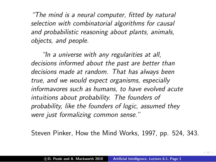
“The mind is a neural computer, fitted by natural selection with combinatorial algorithms for causal and probabilistic reasoning about plants, animals,

• bjects, and people.

“In a universe with any regularities at all, decisions informed about the past are better than decisions made at random. That has always been true, and we would expect organisms, especially informavores such as humans, to have evolved acute intuitions about probability. The founders of probability, like the founders of logic, assumed they were just formalizing common sense.” Steven Pinker, How the Mind Works, 1997, pp. 524, 343.

c

• D. Poole and A. Mackworth 2010

Artificial Intelligence, Lecture 6.1, Page 1

Learning Objectives

At the end of the class you should be able to: justify the use and semantics of probability know how to compute marginals and apply Bayes’ theorem build a belief network for a domain predict the inferences for a belief network explain the predictions of a causal model

c

• D. Poole and A. Mackworth 2010

Artificial Intelligence, Lecture 6.1, Page 2

Using Uncertain Knowledge

Agents don’t have complete knowledge about the world. Agents need to make decisions based on their uncertainty. It isn’t enough to assume what the world is like. Example: wearing a seat belt. An agent needs to reason about its uncertainty.

c

• D. Poole and A. Mackworth 2010

Artificial Intelligence, Lecture 6.1, Page 3

Why Probability?

There is lots of uncertainty about the world, but agents still need to act. Predictions are needed to decide what to do:

◮ definitive predictions: you will be run over tomorrow ◮ point probabilities: probability you will be run over

tomorrow is 0.002

◮ probability ranges: you will be run over with probability

in range [0.001,0.34]

Acting is gambling: agents who don’t use probabilities will lose to those who do — Dutch books. Probabilities can be learned from data. Bayes’ rule specifies how to combine data and prior knowledge.

c

• D. Poole and A. Mackworth 2010

Artificial Intelligence, Lecture 6.1, Page 4

Probability

Probability is an agent’s measure of belief in some proposition — subjective probability. An agent’s belief depends on its prior assumptions and what the agent observes.

c

• D. Poole and A. Mackworth 2010

Artificial Intelligence, Lecture 6.1, Page 5

Numerical Measures of Belief

Belief in proposition, f , can be measured in terms of a number between 0 and 1 — this is the probability of f .

◮ The probability f is 0 means that f is believed to be

definitely false.

◮ The probability f is 1 means that f is believed to be

definitely true.

Using 0 and 1 is purely a convention. f has a probability between 0 and 1, means the agent is ignorant of its truth value. Probability is a measure of an agent’s ignorance. Probability is not a measure of degree of truth.

c

• D. Poole and A. Mackworth 2010

Artificial Intelligence, Lecture 6.1, Page 6

Random Variables

A random variable is a term in a language that can take

• ne of a number of different values.

The range of a variable X, written range(X), is the set

• f values X can take.

A tuple of random variables X1, . . . , Xn is a complex random variable with range range(X1) × · · · × range(Xn). Often the tuple is written as X1, . . . , Xn. Assignment X = x means variable X has value x. A proposition is a Boolean formula made from assignments of values to variables.

c

• D. Poole and A. Mackworth 2010

Artificial Intelligence, Lecture 6.1, Page 7

Possible World Semantics

A possible world specifies an assignment of one value to each random variable. A random variable is a function from possible worlds into the range of the random variable. ω | = X = x means variable X is assigned value x in world ω. Logical connectives have their standard meaning: ω | = α ∧ β if ω | = α and ω | = β ω | = α ∨ β if ω | = α or ω | = β ω | = ¬α if ω | = α Let Ω be the set of all possible worlds.

c

• D. Poole and A. Mackworth 2010

Artificial Intelligence, Lecture 6.1, Page 8

Semantics of Probability

For a finite number of possible worlds: Define a nonnegative measure µ(ω) to each world ω so that the measures of the possible worlds sum to 1. The probability of proposition f is defined by: P(f ) =

• ω|

=f

µ(ω).

c

• D. Poole and A. Mackworth 2010

Artificial Intelligence, Lecture 6.1, Page 9

Axioms of Probability: finite case

Three axioms define what follows from a set of probabilities: Axiom 1 0 ≤ P(a) for any proposition a. Axiom 2 P(true) = 1 Axiom 3 P(a ∨ b) = P(a) + P(b) if a and b cannot both be true. These axioms are sound and complete with respect to the semantics.

c

• D. Poole and A. Mackworth 2010

Artificial Intelligence, Lecture 6.1, Page 10

Semantics of Probability: general case

In the general case, probability defines a measure on sets of possible worlds. We define µ(S) for some sets S ⊆ Ω satisfying: µ(S) ≥ 0 µ(Ω) = 1 µ(S1 ∪ S2) = µ(S1) + µ(S2) if S1 ∩ S2 = {}. Or sometimes σ-additivity: µ(

• i

Si) =

• i

µ(Si) if Si ∩ Sj = {} for i = j Then P(α) = µ({ω|ω | = α}).

c

• D. Poole and A. Mackworth 2010

Artificial Intelligence, Lecture 6.1, Page 11

Probability Distributions

A probability distribution on a random variable X is a function range(X) → [0, 1] such that x → P(X = x). This is written as P(X). This also includes the case where we have tuples of

• variables. E.g., P(X, Y , Z) means P(X, Y , Z).

When range(X) is infinite sometimes we need a probability density function...

c

• D. Poole and A. Mackworth 2010

Artificial Intelligence, Lecture 6.1, Page 12

Conditioning

Probabilistic conditioning specifies how to revise beliefs based on new information. An agent builds a probabilistic model taking all background information into account. This gives the prior probability. All other information must be conditioned on. If evidence e is the all of the information obtained subsequently, the conditional probability P(h|e) of h given e is the posterior probability of h.

c

• D. Poole and A. Mackworth 2010

Artificial Intelligence, Lecture 6.1, Page 13

Semantics of Conditional Probability

Evidence e rules out possible worlds incompatible with e. Evidence e induces a new measure, µe, over possible worlds µe(S) = c × µ(S) if ω | = e for all ω ∈ S if ω | = e for all ω ∈ S We can show c =

c

• D. Poole and A. Mackworth 2010

Artificial Intelligence, Lecture 6.1, Page 14

Semantics of Conditional Probability

Evidence e rules out possible worlds incompatible with e. Evidence e induces a new measure, µe, over possible worlds µe(S) = c × µ(S) if ω | = e for all ω ∈ S if ω | = e for all ω ∈ S We can show c =

1 P(e).

The conditional probability of formula h given evidence e is P(h|e) = µe({ω : ω | = h}) =

c

• D. Poole and A. Mackworth 2010

Artificial Intelligence, Lecture 6.1, Page 15

Semantics of Conditional Probability

Evidence e rules out possible worlds incompatible with e. Evidence e induces a new measure, µe, over possible worlds µe(S) = c × µ(S) if ω | = e for all ω ∈ S if ω | = e for all ω ∈ S We can show c =

1 P(e).

The conditional probability of formula h given evidence e is P(h|e) = µe({ω : ω | = h}) = P(h ∧ e) P(e)

c

• D. Poole and A. Mackworth 2010

Artificial Intelligence, Lecture 6.1, Page 16

Conditioning

Possible Worlds:

c

• D. Poole and A. Mackworth 2010

Artificial Intelligence, Lecture 6.1, Page 17

Conditioning

Possible Worlds: Observe Color = orange:

c

• D. Poole and A. Mackworth 2010

Artificial Intelligence, Lecture 6.1, Page 18

Exercise

Flu Sneeze Snore µ true true true 0.064 true true false 0.096 true false true 0.016 true false false 0.024 false true true 0.096 false true false 0.144 false false true 0.224 false false false 0.336 What is: (a) P(flu ∧ sneeze) (b) P(flu ∧ ¬sneeze) (c) P(flu) (d) P(sneeze | flu) (e) P(¬flu ∧ sneeze) (f) P(flu | sneeze) (g) P(sneeze | flu∧snore) (h) P(flu | sneeze∧snore)

c

• D. Poole and A. Mackworth 2010

Artificial Intelligence, Lecture 6.1, Page 19

Chain Rule

P(f1 ∧ f2 ∧ . . . ∧ fn) =

c

• D. Poole and A. Mackworth 2010

Artificial Intelligence, Lecture 6.1, Page 20

Chain Rule

P(f1 ∧ f2 ∧ . . . ∧ fn) = P(fn|f1 ∧ · · · ∧ fn−1) × P(f1 ∧ · · · ∧ fn−1) =

c

• D. Poole and A. Mackworth 2010

Artificial Intelligence, Lecture 6.1, Page 21

Chain Rule

P(f1 ∧ f2 ∧ . . . ∧ fn) = P(fn|f1 ∧ · · · ∧ fn−1) × P(f1 ∧ · · · ∧ fn−1) = P(fn|f1 ∧ · · · ∧ fn−1) × P(fn−1|f1 ∧ · · · ∧ fn−2) × P(f1 ∧ · · · ∧ fn−2) = P(fn|f1 ∧ · · · ∧ fn−1) × P(fn−1|f1 ∧ · · · ∧ fn−2) × · · · × P(f3|f1 ∧ f2) × P(f2|f1) × P(f1) =

n

• i=1

P(fi|f1 ∧ · · · ∧ fi−1)

c

• D. Poole and A. Mackworth 2010

Artificial Intelligence, Lecture 6.1, Page 22

Bayes’ theorem

The chain rule and commutativity of conjunction (h ∧ e is equivalent to e ∧ h) gives us: P(h ∧ e) =

c

• D. Poole and A. Mackworth 2010

Artificial Intelligence, Lecture 6.1, Page 23

Bayes’ theorem

The chain rule and commutativity of conjunction (h ∧ e is equivalent to e ∧ h) gives us: P(h ∧ e) = P(h|e) × P(e)

c

• D. Poole and A. Mackworth 2010

Artificial Intelligence, Lecture 6.1, Page 24

Bayes’ theorem

The chain rule and commutativity of conjunction (h ∧ e is equivalent to e ∧ h) gives us: P(h ∧ e) = P(h|e) × P(e) = P(e|h) × P(h).

c

• D. Poole and A. Mackworth 2010

Artificial Intelligence, Lecture 6.1, Page 25

Bayes’ theorem

The chain rule and commutativity of conjunction (h ∧ e is equivalent to e ∧ h) gives us: P(h ∧ e) = P(h|e) × P(e) = P(e|h) × P(h). If P(e) = 0, divide the right hand sides by P(e): P(h|e) =

c

• D. Poole and A. Mackworth 2010

Artificial Intelligence, Lecture 6.1, Page 26

Bayes’ theorem

The chain rule and commutativity of conjunction (h ∧ e is equivalent to e ∧ h) gives us: P(h ∧ e) = P(h|e) × P(e) = P(e|h) × P(h). If P(e) = 0, divide the right hand sides by P(e): P(h|e) = P(e|h) × P(h) P(e) . This is Bayes’ theorem.

c

• D. Poole and A. Mackworth 2010

Artificial Intelligence, Lecture 6.1, Page 27

Why is Bayes’ theorem interesting?

Often you have causal knowledge: P(symptom | disease) P(light is off | status of switches and switch positions) P(alarm | fire) P(image looks like | a tree is in front of a car) and want to do evidential reasoning: P(disease | symptom) P(status of switches | light is off and switch positions) P(fire | alarm). P(a tree is in front of a car | image looks like )

c

• D. Poole and A. Mackworth 2010

Artificial Intelligence, Lecture 6.1, Page 28

Exercise

A cab was involved in a hit-and-run accident at night. Two cab companies, the Green and the Blue, operate in the city. You are given the following data: 85% of the cabs in the city are Green and 15% are Blue. A witness identified the cab as Blue. The court tested the reliability of the witness in the circumstances that existed

• n the night of the accident and concluded that the

witness correctly identifies each one of the two colours 80% of the time and failed 20% of the time. What is the probability that the cab involved in the accident was Blue?

c

• D. Poole and A. Mackworth 2010

Artificial Intelligence, Lecture 6.1, Page 29

Exercise

A cab was involved in a hit-and-run accident at night. Two cab companies, the Green and the Blue, operate in the city. You are given the following data: 85% of the cabs in the city are Green and 15% are Blue. A witness identified the cab as Blue. The court tested the reliability of the witness in the circumstances that existed

• n the night of the accident and concluded that the

witness correctly identifies each one of the two colours 80% of the time and failed 20% of the time. What is the probability that the cab involved in the accident was Blue? From D. Kahneman, Thinking Fast and Slow, 2011, p. 166.

c

• D. Poole and A. Mackworth 2010

Artificial Intelligence, Lecture 6.1, Page 30

Exercise

A cab was involved in a hit-and-run accident at night. Two cab companies, the Green and the Blue, operate in the city. You are given the following data: The two companies operate the same number of cabs, but Green cabs are involved in 85% of the accidents. A witness identified the cab as Blue. The court tested the reliability of the witness in the circumstances that existed

• n the night of the accident and concluded that the

witness correctly identifies each one of the two colours 80% of the time and failed 20% of the time. What is the probability that the cab involved in the accident was Blue?

c

• D. Poole and A. Mackworth 2010

Artificial Intelligence, Lecture 6.1, Page 31

Exercise

A cab was involved in a hit-and-run accident at night. Two cab companies, the Green and the Blue, operate in the city. You are given the following data: The two companies operate the same number of cabs, but Green cabs are involved in 85% of the accidents. A witness identified the cab as Blue. The court tested the reliability of the witness in the circumstances that existed

• n the night of the accident and concluded that the

witness correctly identifies each one of the two colours 80% of the time and failed 20% of the time. What is the probability that the cab involved in the accident was Blue? From D. Kahneman, Thinking Fast and Slow, 2011, p. 167. Chapter 16 “Causes trump statistics”

c

• D. Poole and A. Mackworth 2010

Artificial Intelligence, Lecture 6.1, Page 32