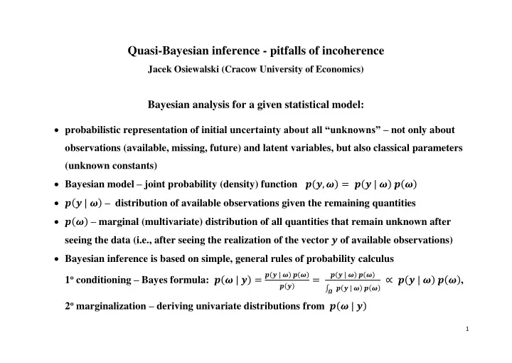
Quasi-Bayesian inference - pitfalls of incoherence Jacek Osiewalski - PowerPoint PPT Presentation

Quasi-Bayesian inference - pitfalls of incoherence Jacek Osiewalski (Cracow University of Economics) Bayesian analysis for a given statistical model:  probabilistic representation of initial un certainty about all “unknowns” – not only about observations (available, missing, future) and latent variables, but also classical parameters (unknown constants)  Bayesian model – joint probability (density) function 𝒒(𝒛, 𝝏) = 𝒒(𝒛 | 𝝏) 𝒒(𝝏)  𝒒(𝒛 | 𝝏) – distribution of available observations given the remaining quantities  𝒒(𝝏) – marginal (multivariate) distribution of all quantities that remain unknown after seeing the data (i.e., after seeing the realization of the vector 𝒛 of available observations)  Bayesian inference is based on simple, general rules of probability calculus 𝒒(𝒛 | 𝝏) 𝒒(𝝏) 𝒒(𝒛 | 𝝏) 𝒒(𝝏) 1 o conditioning – Bayes formula: 𝒒(𝝏 | 𝒛) = ∝ 𝒒(𝒛 | 𝝏) 𝒒(𝝏) , = 𝒒(𝒛) 𝒒(𝒛 | 𝝏) 𝒒(𝝏) ∫ 𝜵 2 o marginalization – deriving univariate distributions from 𝒒(𝝏 | 𝒛) 1

“ Coherent inference ” – the one following strict rules of probability calculus Quasi-Bayesian inference:  Bayes formula used mechanically, outside the full probabilistic context – incoherence !  𝒒(𝒛 | 𝝏) = 𝒉(𝒛; 𝝏) corresponds to some traditional statistical model  𝒒(𝝏) = 𝒈(𝝏; 𝒛) is specified using given 𝒛 , so it cannot be the marginal distribution !!!  thus 𝒒(𝝏 | 𝒛) ∝ 𝒉(𝒛; 𝝏) 𝒈(𝝏; 𝒛) IS NOT the posterior in a Bayesian model with initially assumed 𝒒(𝒛 | 𝝏) , but it can be the posterior in a completely different Bayesian model  question: what are the true building blocks (statistical model and prior) corresponding to such 𝒒(𝝏 | 𝒛) ? it would be useful to know true assumptions, not only the declared ones  fundamental pitfall of incoherence – 𝒒(𝝏 | 𝒛) corresponds to some statistical model and prior assumptions to be discovered ! So- called “Empirical Bayes” (EB) is the most popular quasi-Bayesian approach, advocated in non-Bayesian, sampling-theory texts on inference in hierarchical multi-level statistical models → Here we show hidden assumptions behind the EB inference in hierarchical models 2

SOME SIMPLE EXAMPLE FIRST (Example 1) 𝟐 (𝝂 | 𝒃, 𝒘) 𝒐 (𝒛 | 𝝂 𝒇 𝒐 , 𝒅𝑱 𝒐 )𝒈 𝑶 𝒒(𝒛, 𝝂) = 𝒒(𝒛 | 𝝂) 𝒒(𝝂) = 𝒈 𝑶 Bayesian model: ′ )𝒈 𝑶 𝟐 (𝝂 | 𝒃 𝒛 , 𝒘 𝒛 ) 𝒐 (𝒛 | 𝒃 𝒇 𝒐 , 𝒅𝑱 𝒐 + 𝒘 𝒇 𝒐 𝒇 𝒐 𝒒(𝒛, 𝝂) = 𝒒(𝒛) 𝒒(𝝂 | 𝒛) = 𝒈 𝑶 Decomposition: −𝟐 −𝟐 ′ 𝒛 , 𝒇 𝒐 = (𝟐 𝟐 … 𝟐)′ 𝒐 𝟐 𝒐 𝟐 𝒐 𝟐 𝟐 𝒘 𝒛 = ( 𝒅 + 𝒘 ) , 𝒃 𝒛 = ( 𝒅 + 𝒘 ) ( 𝒅 𝒛 ̅ + 𝒘 𝒃), 𝒛 ̅ = 𝒐 𝒇 𝒐 where Quasi-Bayesian inference: imagine a non-Bayesian statistician who agrees to use Bayes formula 𝒒(𝝂 | 𝒛) ∝ 𝒒(𝒛 | 𝝂) 𝒒(𝝂) but disagrees to subjectively specify 𝒃 (prior mean); instead he/she puts 𝒛 ̅ (sample average) −𝟐 𝟐 (𝝂 | 𝒛 𝟐 (𝝂 | 𝒛 𝒐 𝟐 𝒒 ∗ (𝝂) = 𝒈 𝑶 ̅, 𝒘) and 𝒒 ∗ (𝝂 | 𝒛) = 𝒈 𝑶 ̅, ( 𝒅 + 𝒘 ) ) and (informally) uses Is there any hidden Bayesian model (sampling + prior) formally justifying such “posterior”? 𝟐 (𝝂 − 𝒛 𝒐 (𝒛 − 𝝂 𝒇 𝒐 | 𝟏, 𝒅𝑱 𝒐 ) 𝒈 𝑶 ̃(𝒛, 𝝂) = 𝒒(𝒛 | 𝝂) 𝒒 ∗ (𝝂) = 𝒈 𝑶 𝒒 ̅ | 𝟏, 𝒘) Consider 𝟐 𝟐 ̃(𝝂 | 𝒛) = 𝒒 ∗ (𝝂 | 𝒛) and 𝒒 𝟑𝒅 𝒛 ′ 𝑵𝒛) , 𝑵 = 𝑱 𝒐 − ′ ̃(𝒛) ∝ 𝐟𝐲𝐪 (− 𝒒 𝒐 𝒇 𝒐 𝒇 𝒐 it decomposes into 𝒐 (𝒛 | 𝝂 𝒇 𝒐 , 𝒅 (𝑱 𝒐 − ′ )) and 𝒒 𝒅 ̃(𝒛 | 𝝂) = 𝒈 𝑶 ̃(𝝂) constant (!!!) or 𝒒 𝒐(𝒅+𝒐𝒘) 𝒇 𝒐 𝒇 𝒐 true sampling model assumes dependence (equi-correlation); true prior is flat, improper 3

MAIN PART: Statistical models with hierarchical structure 𝒒(𝒛|𝜾) = 𝒉(𝒛; 𝜾), 𝒛𝝑𝒁, 𝜾𝝑𝚰; conditional distribution of observations: 𝒈 𝟏 (𝜾; 𝜷), 𝜷𝝑𝑩 ⊆ ℝ 𝒕 ; distribution of random parameters (latent variables): joint distribution ( α fixed): 𝒒(𝒛|𝜾) 𝒈 𝟏 (𝜾; 𝜷) = 𝒉(𝒛; 𝜾) 𝒈 𝟏 (𝜾; 𝜷) = 𝒈 𝟐 (𝜾|𝒛; 𝜷) 𝒊(𝒛; 𝜷)  decomposition 𝒊(𝒛; 𝜷)  marginal distribution of 𝒛 𝒉(𝒛;𝜾) 𝒈 𝟏 (𝜾;𝜷) 𝒈 𝟐 (𝜾|𝒛; 𝜷) = ∝ 𝒉(𝒛; 𝜾) 𝒈 𝟏 (𝜾; 𝜷)  conditional distribution of 𝜾 (Bayes formula) 𝒊(𝒛;𝜷) 4

SIMPLE EXAMPLE OF A HIERARCHICAL MODEL (Example 2) 𝜾 𝒋 – unobservable characteristic, randomly distributed over 𝒐 observed units (𝒋 = 𝟐, … , 𝒐) , 𝜾 = (𝜾 𝟐 … 𝜾 𝒐 ) ′ , 𝜾 𝒋 ~𝒋𝒋𝑶(𝜷, 𝒆), 𝒆 > 𝟏 known; 𝒚 𝒋 = (𝒚 𝒋𝟐 … 𝒚 𝒋𝒏 ) ′ , 𝒚 𝒋𝒌 ~𝒋𝒋𝑶(𝜾 𝒋 , 𝒅 𝟏 ) (𝒌 = 𝟐, … , 𝒏) – independent measurements of 𝜾 𝒋 ( 𝒅 𝟏 known) ′ 𝒚 𝒋 = 𝒚 𝟐 𝒅 𝟏 ̅ 𝒋. – sufficient statistic (for fixed 𝜾 𝒋 ); 𝒛 𝒋 ~𝒋𝒋𝑶(𝜾 𝒋 , 𝒅), 𝒅 = 𝒛 𝒋 = 𝒏 𝒇 𝒏 𝒏 , 𝒛 = (𝒛 𝟐 … 𝒛 𝒐 )′ 𝒐 (𝒛|𝜾, 𝒅𝑱 𝒐 ), 𝒈 𝟏 (𝜾; 𝜷) = 𝒈 𝑶 𝒐 (𝜾|𝜷𝒇 𝒐 , 𝒆𝑱 𝒐 ) 𝒒(𝒛|𝜾) = 𝒈 𝑶 Decomposition of the product 𝒒(𝒛|𝜾) 𝒈 𝟏 (𝜾; 𝜷) into 𝒈 𝟐 (𝜾|𝒛; 𝜷) 𝒊(𝒛; 𝜷) , where 𝒐 (𝒛|𝜷𝒇 𝒐 , (𝒅 + 𝒆)𝑱 𝒐 ) , 𝒊(𝒛; 𝜷) = ∫ 𝒒(𝒛|𝜾) 𝒈 𝟏 (𝜾; 𝜷) 𝒆𝜾 = 𝒈 𝑶 ℝ 𝒐 𝒆 −𝟐 𝒅 −𝟐 𝟐 𝒐 (𝜾| 𝒈 𝟐 (𝜾|𝒛; 𝜷) = 𝒈 𝑶 𝒅 −𝟐 +𝒆 −𝟐 𝜷𝒇 𝒐 + 𝒅 −𝟐 +𝒆 −𝟐 𝒛, 𝒅 −𝟐 +𝒆 −𝟐 𝑱 𝒐 ) (final precision = sample + prior) 𝒆 −𝟐 𝑭(𝜾|𝒛; 𝜷) = 𝒙 ∙ 𝜷𝒇 𝒐 + (𝟐 − 𝒙) ∙ 𝒛, 𝒙 = 𝒅 −𝟐 +𝒆 −𝟐 𝝑(𝟏, 𝟐) ( 𝒙 = prior precision / final precision) 𝑭(𝜾|𝒛; 𝜷) – point in 𝚰 = ℝ 𝒐 lying on the line segment between (𝜷 𝜷 … 𝜷)′ and (𝒛 𝟐 𝒛 𝟑 … 𝒛 𝒐 )′ 𝒈 𝟐 (𝜾|𝒛; 𝜷) follows Bayes Theorem for any fixed 𝜷 , so then we have coherence; but how to get 𝜷 ? 5

Empirical Bayes (EB) inference on 𝜾 based on the conditional distribution 𝒈 𝟐 (𝜾|𝒛; 𝜷) obtained using Bayes Theorem, BUT for some point estimate of unknown 𝜷𝝑𝑩 , e.g., using so-called type II maximum likelihood: ̂ = 𝜷 ̂ 𝑵𝑴 = 𝐛𝐬𝐡 𝐧𝐛𝐲 𝑴(𝜷; 𝒛) = 𝐛𝐬𝐡 𝐧𝐛𝐲 𝒊(𝒛; 𝜷), 𝜷𝝑𝑩 𝜷 𝒒 ̂(𝜾|𝒛) = 𝒈 𝟐 (𝜾|𝒛, 𝜷 ̂) ∝ 𝒒(𝒛|𝜾)𝒈 𝟏 (𝜾; 𝜷 ̂) , So EB uses i.e. the “posterior” corresponding to the “prior” with hyper-parameter based on 𝒛 !!! EXAMPLE 2 (continued) 𝟐 𝟐 (𝜷|𝒛 𝒅+𝒆 𝒅+𝒆 𝒐 (𝒛|𝜷𝒇 𝒐 , (𝒅 + 𝒆)𝑱 𝒐 ) = (𝟑𝝆 ∙ 𝒐 (𝑵𝒛|𝟏, (𝒅 + 𝒆)𝑱 𝒐 ) , 𝑴(𝜷; 𝒛) = 𝒊(𝒛; 𝜷) = 𝒈 𝑶 𝒐 ) 𝟑 𝒈 𝑶 ̅, 𝒐 ) 𝒈 𝑶 ′ 𝒛 , 𝟐 𝟐 ′ , ̂ = 𝜷 ̂ 𝑵𝑴 = 𝒛 ̅ = 𝜷 𝒐 𝒇 𝒐 𝑵 = 𝑱 𝒐 − 𝒐 𝒇 𝒐 𝒇 𝒐 𝒆 −𝟐 𝒅 −𝟐 𝟐 ̂ 𝑭𝑪 , ̂ 𝑭𝑪 = 𝒐 (𝜾|𝜾 ̂(𝜾|𝒛) = 𝒈 𝟐 (𝜾|𝒛, 𝜷 ̂) = 𝒈 𝑶 ̅𝒇 𝒐 + 𝒒 𝒅 −𝟐 +𝒆 −𝟐 𝑱 𝒐 ) , 𝜾 𝒅 −𝟐 +𝒆 −𝟐 𝒛 𝒅 −𝟐 +𝒆 −𝟐 𝒛  uncertainty about 𝜷 not taken into account  obvious incoherence of inferences on 𝜾 6

Bayesian hierarchical model (BHM) 𝒒(𝒛, 𝝏) = 𝒒(𝒛, 𝜾, 𝜷) = 𝒒(𝒛|𝜾) 𝒒(𝜾|𝜷) 𝒒(𝜷), 𝒒(𝜷) – the prior for 𝜷𝝑𝑩 𝝏 = (𝜾, 𝜷) , conditional independence: 𝒛 ⊥ 𝜷 | 𝜾 – leads to 𝒒(𝒛|𝝏) = 𝒒(𝒛|𝜾) 𝒒(𝒛|𝜾) = 𝒉(𝒛; 𝜾), 𝒒(𝜾|𝜷) = 𝒈 𝟏 (𝜾; 𝜷) – the same as in EB final decomposition of Bayesian model: 𝒒(𝒛, 𝜾, 𝜷) = 𝒒(𝒛) 𝒒(𝜾, 𝜷|𝒛) = 𝒒(𝒛) 𝒒(𝜷|𝒛) 𝒒(𝜾|𝒛, 𝜷) 𝒒(𝜾|𝒛, 𝜷) = 𝒒(𝒛|𝜾) 𝒒(𝜾|𝜷) = 𝒉(𝒛; 𝜾) 𝒈 𝟏 (𝜾; 𝜷) = 𝒈 𝟐 (𝜾|𝒛; 𝜷) 𝒒(𝒛|𝜷) 𝒊(𝒛; 𝜷) 𝒒(𝜷|𝒛) = 𝒒(𝒛|𝜷) 𝒒(𝜷) = 𝒊(𝒛; 𝜷) 𝒒(𝜷) 𝒒(𝒛) 𝒒(𝒛) 𝒒(𝒛) = ∫ 𝒒(𝒛|𝜷 ) 𝒒(𝜷) 𝒆𝜷 𝑩 Remarks:  𝒒(𝜾|𝒛) = ∫ 𝒈 𝟐 (𝜾|𝒛; 𝜷) 𝒒(𝜷|𝒛) 𝒆𝜷 – uncertainty about 𝜷 is formally taken into account 𝑩  Bayes Theorem is used twice: for latent variables (given parameters) and for parameters 7