SELECTION Deterministic Stochastic Proportionate selection: - PDF document
SELECTION Deterministic Stochastic Proportionate selection: Roulette Wheel Selection Rank based selection Tournament Selection COMPETITION (mu) denotes the size of the (parent) population (lambda) denotes the
SELECTION • Deterministic • Stochastic – Proportionate selection: Roulette Wheel Selection – Rank based selection – Tournament Selection
COMPETITION • µ (mu) denotes the size of the (parent) population • λ (lambda) denotes the number of offspring produced • ( µ, λ ) competition: new population is formed exclusively from offspring (aka Generational EA) • ( µ + λ ) competition: new population is formed from old population (parents) and offspring (called Steady State EA when λ << µ )
Travelling Salesperson Problem (TSP) • Problem: given x cities, what is the short- est tour in which each city is visited once and only once? • NP-hard: no known algorithm which is a polynomial function of the number of cities • Example applications – Circuit board drilling (17,000 cities) – X-ray crystallography (14,000 cities) – VLSI fabrication (1.2 million cities) • Trial solution representation: permutation of integers
• Fitness function: straightforward • Genetic operators: not obvious
Boolean Satisfiability Problem (SAT) • Given a compound Boolean statement, find a set of truth assignments such that the statement evaluates to TRUE. • NP-complete: NP-hard and NP • Trial solution representation: binary string • Fitness function: not obvious • Genetic operators: crossover and mutation
Theoretical Foundations of Genetic Algorithms • Schema - a template allowing exploration of similarities among individuals (binary strings) • A schema consists of 0’s, 1’s and *’s (don’t care symbol) • One particular schema represents all strings (a hyperplane or subset of the search space) which match it on all positions other than ‘*’ • Every schema matches exactly 2 r strings, where r is the number of *’s • Each string of length m is matched by 2 m schemata
• For length m there are 3 m possible schemata • The order of schema S (denoted by o ( S )) is the number of fixed positions (non- don ′ t care positions) in S (= m − r ) • The defining length of schema S (denoted by δ ( S )) is the distance between the first and the last fixed string positions (it de- fines the compactness of information con- tained in a schema) • The number of strings in a population at time t matched by schema S is denoted by ξ ( S, t ) • The fitness of a schema at time t , eval ( S, t ), is defined as the average fitness of all strings in the population matched by the schema S
• Population consists of strings { v 1 , · · · , v popsize } • Given p strings { v i 1 , · · · , v i p } in population matched by schema S i , then: p � eval ( S i , t ) = eval ( v i j ) /p (1) j =1 • Total fitness of population F ( t ) = � popsize eval ( v i ) i =1 • Assume generational model with propor- tional (roulette wheel) selection • Single string selection chance: eval ( v i ) /F ( t ) • Selection chance for average string matched by schema S : eval ( S, t ) /F ( t )
• Combining the above we get: E [ ξ ( S, t +1)] = ξ ( S, t ) · popsize · eval ( S, t ) /F ( t ) (2) • Average population fitness F ( t ) = F ( t ) /popsize • Reproductive schema growth equation: E [ ξ ( S, t + 1)] = ξ ( S, t ) · eval ( S, t ) /F ( t ) (3) • If schema S remains above average by ǫ %, in other words eval ( S, t ) = (1 + ǫ ) · F ( t ), then we obtain the following geometric pro- gression equation: E [ ξ ( S, t )] = ξ ( S, 0)(1 + ǫ ) t (4) • Now assume 1-point crossover with crossover chance p c ; a crossover point is selected uni- formly among m − 1 possible locations
• Probability of schema destruction: p d ( S ) ≤ p c · δ ( S ) (5) m − 1 • Consequently, probability of schema sur- vival: p s ( S ) ≥ 1 − p c · δ ( S ) (6) m − 1 • New reproductive schema growth equation: � � E [ ξ ( S, t +1)] ≥ ξ ( S, t ) · eval ( S, t ) 1 − p c · δ ( S ) m − 1 F ( t ) (7) • Finally, add mutation with bit mutation chance p m ; single bit survival is 1 − p m • Schema survival p s ( S ) = (1 − p m ) o ( S )
• Since p m ≪ 1, schema survival can be ap- proximated as p s ( S ) ≈ 1 − o ( S ) · p m • Combined reproductive schema growth equa- tion: E [ ξ ( S, t + 1)] ≥ � � ξ ( S, t ) · eval ( S, t ) 1 − p c · δ ( S ) m − 1 − o ( S ) · p m F ( t ) (8) • Schema Theorem: Short, low-order, above- average schemata receive exponentially in- creasing trials in subsequent generations of a genetic algorithm
• Building Block Hypothesis: A genetic algo- rithm seeks near-optimal performance through the juxtaposition of short, low-order, high- performance schemata, called the building blocks • Consequence: the manner in which we en- code a problem is critical for the perfor- mance of a GA - it should satisfy the idea of short building blocks
GRAY CODING • Desired: points close to each other in rep- resentation space also close to each other in problem space • This is not the case when binary numbers represent floating point values • m is number of bits in representation • binary number � b = ( b 1 , b 2 , · · · , b m ) • Gray code number � g = ( g 1 , g 2 , · · · , g m )
binary gray code 000 000 001 001 010 011 011 010 100 110 101 111 110 101 111 100 PROCEDURE Binary-To-Gray g 1 ⇐ b 1 for k = 2 to m do g k ⇐ b k − 1 XOR b k end for
PROCEDURE Gray-To-Binary value ⇐ g 1 b 1 ⇐ value for k = 2 to m do if g k = 1 then value ⇐ NOT value end if b k ⇐ value end for
Evolution of Evolution Strategies • Earliest ES had popsize = 1 and the sole genetic operator employed was mutation • EC literature often refers to the (1+1) ES as “two-membered evolution strategy” • Individual represented as pair of float-valued vectors ( x, σ ), with x representing a point in search space and σ a vector of standard deviations • Mutation: x t +1 = x t + N (0 , σ ) where N (0 , σ ) is a vector of independent random Gaus- sian numbers with a mean of zero and stan- dard deviations σ
offspring ( x t +1 , σ ) replaces • Competition: its parent ( x t , σ ) iff fitness ( x t +1 ) > fitness ( x t ) • If all components of σ are identical and the optimization problem is regular , it is pos- sible to prove the Convergence Theorem: For σ > 0 and a regular optimization prob- lem, t →∞ f ( x t ) = f opt } = 1 p { lim • Optimize convergence rate with Rechen- berg’s “1/5 success rule”: The ratio ϕ of successful mutations to all mutations should be 1/5. Increase the vari- ance of the mutation operator if ϕ is greater than 1/5, otherwise decrease it.
• Applying the 1/5 rule every k generations can be performed as follows: c d · σ t if ϕ ( k ) < 1 / 5 σ t +1 = c i · σ t if ϕ ( k ) > 1 / 5 σ t if ϕ ( k ) = 1 / 5 where ϕ ( k ) is the mutation success ratio during the last k generations. Schwefel used in a number of his experiments the following values: c d = 0 . 82 and c i = 1 . 22(= 1 / 0 . 82) • For some classes of functions this rule lead to premature convergence; solution: in- creased population size • EC literature often refers to an ( µ + 1)-ES as “multi-membered evolution strategy” • All individuals have equal mating probabil- ities
• Recombination can be added in the form of uniform crossover • Further ES evolution lead to the ( µ + λ )-ES and the ( µ, λ )-ES • The deterministic 1/5 rule was replaced by a stochastic process: σ t +1 = σ t · e N (0 , ∆ σ ) where ∆ σ is a parameter of the process
Recommend
More recommend
Explore More Topics
Stay informed with curated content and fresh updates.
