Part 9: Text Classification; The Nave Bayes algorithm Francesco - PowerPoint PPT Presentation
Part 9: Text Classification; The Nave Bayes algorithm Francesco Ricci Most of these slides comes from the course: Information Retrieval and Web Search, Christopher Manning and Prabhakar Raghavan 1 Content p Introduction to Text
Part 9: Text Classification; The Naïve Bayes algorithm Francesco Ricci Most of these slides comes from the course: Information Retrieval and Web Search, Christopher Manning and Prabhakar Raghavan 1
Content p Introduction to Text Classification p Bayes rule p Naïve Bayes text classification p Feature independence assumption p Multivariate and Multinomial approaches p Smoothing (avoid overfitting) p Feature selection n Chi square and Mutual Information p Evaluating NB classification. 2
Standing queries p The path from information retrieval to text classification: n You have an information need, say: p "Unrest in the Niger delta region" n You want to rerun an appropriate query periodically to find new news items on this topic n You will be sent new documents that are found p I.e., it ’ s classification not ranking p Such queries are called standing queries n Long used by “ information professionals ” n A modern mass instantiation is Google Alerts. 4
Google alerts 5
Spam filtering: Another text classification task From: "" <takworlld@hotmail.com> Subject: real estate is the only way... gem oalvgkay Anyone can buy real estate with no money down Stop paying rent TODAY ! There is no need to spend hundreds or even thousands for similar courses I am 22 years old and I have already purchased 6 properties using the methods outlined in this truly INCREDIBLE ebook. Change your life NOW ! ================================================= Click Below to order: http://www.wholesaledaily.com/sales/nmd.htm ================================================= 6
Categorization/Classification p Given: n A description of an instance , x ∈ X , where X is the instance language or instance space p Issue: how to represent text documents – the representation determines what information is used for solving the classification task n A fixed set of classes : C = { c 1 , c 2 ,…, c J } p Determine: n The class of x : c ( x ) ∈ C, where c ( x ) is a classification function whose domain is X and whose range is C p We want to know how to build classification functions ( “ classifiers ” ). 7
Document Classification “ planning language Test proof Data: intelligence ” (AI) (Programming) (HCI) Classes: ML Planning Semantics Garb.Coll. Multimedia GUI Training learning planning programming garbage ... ... Data: intelligence temporal semantics collection algorithm reasoning language memory reinforcement plan proof... optimization network... language... region... (Note: in real life there is often a hierarchy, not present in the above problem statement; and also, 8 you get papers on "ML approaches to Garb. Coll.")
More Text Classification Examples p Many search engine functionalities use classification p Assign labels to each document or web-page: n Labels are most often topics such as Yahoo-categories e.g., "finance," "sports," "news>world>asia>business" n Labels may be genres e.g., "editorials" "movie-reviews" "news “ n Labels may be opinion on a person/product e.g., “ like ” , “ hate ” , “ neutral ” n Labels may be domain-specific e.g., "interesting-to-me" : "not-interesting-to-me ” e.g., “ contains adult language ” : “ doesn ’ t ” e.g., language identification: English, French, Chinese, … e.g., “ link spam ” : “ not link spam ” e.g., "key-phrase" : "not key-phrase" 9
Classification Methods (1) p Manual classification n Used by Yahoo! (originally; now present but downplayed), Looksmart, about.com, ODP, PubMed n Very accurate when job is done by experts n Consistent when the problem size and team is small n Difficult and expensive to scale p Means we need automatic classification methods for big problems. 10
Classification Methods (2) p Hand-coded rule-based systems n One technique used by CS dept ’ s spam filter, Reuters, CIA, etc. n Companies (Verity) provide “ IDE ” for writing such rules n Example: assign category if document contains a given Boolean combination of words n Standing queries: Commercial systems have complex query languages (everything in IR query languages + accumulators) n Accuracy is often very high if a rule has been carefully refined over time by a subject expert n Building and maintaining these rules is expensive! 11
Verity topic (a classification rule) p Note: n maintenance issues (author, etc.) n Hand-weighting of terms n But it is easy to explain the results. 12
Classification Methods (3) p Supervised learning of a document-label assignment function p Many systems partly rely on machine learning (Autonomy, MSN, Verity, Enkata, Yahoo!, …) n k-Nearest Neighbors (simple, powerful) n Naive Bayes (simple, common method) n Support-vector machines (new, more powerful) n … plus many other methods p No free lunch: requires hand-classified training data p Note that many commercial systems use a mixture of methods. 13
Recall a few probability basics p For events a and b: p Bayes ’ Rule p ( a , b ) = p ( a ∩ b ) = p ( a | b ) p ( b ) = p ( b | a ) p ( a ) Prior p ( a | b ) = p ( b | a ) p ( a ) p ( b | a ) p ( a ) = ∑ p ( b ) p ( b | x ) p ( x ) x = a , a Posterior p Odds: p ( a ) p ( a ) O ( a ) = = p ( a ) 1 p ( a ) − 14
Bayes ’ Rule Example P ( C , E ) = P ( C | E ) P ( E ) = P ( E | C ) P ( C ) P ( C | E ) = P ( E | C ) P ( C ) P ( E ) P(pass exam | attend classes) = ? = P(pass exam) * P(attend classes | pass exam)/P(attend classes) = 0.7 * 0.9/0.78 Initial estimation = 0.7 * 1.15 = 0.81 Correction based on a ratio 15
Example explained Pass 70% Not pass 30% Attend 50% Attend 90% = P(attend|pass) Not attend 50% Not attend 10% P(pass) = 0.7 P(attend) = P(attend| pass)P(pass) + P(attend | not pass)P(not pass) = 0.9*0.7 + 0.5*0.3 = 0.63 + 0.15 = 0.78 p(pass | attend) = p(pass)*p(attend | pass)/p(attend) 16 = 0.7 * 0.9/0.78 = 0.81
Bayesian Methods p Our focus this lecture p Learning and classification methods based on probability theory p Bayes theorem plays a critical role in probabilistic learning and classification p Uses prior probability of each category given no information about an item p Obtains a posterior probability distribution over the possible categories given a description of an item . 17
Naive Bayes Classifiers p Task: Classify a new instance D based on a tuple of attribute values into one of D x , x , … , x = 1 2 n the classes c j ∈ C P ( c j | x 1 , x 2 , … , x n ) c MAP = argmax c j ∈ C P ( x , x , … , x | c ) P ( c ) Maximum A 1 2 n j j argmax = Posteriori P ( x , x , … , x ) c C ∈ class 1 2 n j argmax P ( x , x , … , x | c ) P ( c ) = 1 2 n j j c C ∈ j 18
Naïve Bayes Assumption p P ( c j ) n Can be estimated from the frequency of classes in the training examples p P ( x 1 ,x 2 ,…,x n |c j ) n O( |X| n |C| ) parameters ( assuming X finite ) n Could only be estimated if a very, very large number of training examples was available – or? p Naïve Bayes Conditional Independence Assumption: n Assume that the probability of observing the conjunction of attributes is equal to the product of the individual probabilities P ( x i | c j ). n ∏ c MAP = argmax P ( c j ) P ( x i | c j ) 19 c j ∈ C i = 1
The Naïve Bayes Classifier Flu X 1 X 2 X 3 X 4 X 5 runnynose sinus cough fever muscle-ache p Conditional Independence Assumption: features detect term presence and are independent of each other given the class: P ( x 1 , … , x 5 | C ) = P ( x 1 | C ) • P ( x 2 | C ) • • P ( x 5 | C ) p This model is appropriate for binary variables = many n Multivariate Bernoulli model variables 20 =only 2 values – T or F
Learning the Model C X 1 X 2 X 3 X 4 X 5 X 6 p First attempt: maximum likelihood estimates n simply use the frequencies in the data N ( C c ) = ˆ j P ( c ) Estimated conditional = j probability that the N attribute X i (e.g. Fever) has the value x i (True or N ( X x , C c ) = = ˆ False) – we will also write i i j P ( x | c ) = P(Fever | c j ) instead of i j N ( C c ) = 21 P(Fever = T | c j ) j
Problem with Max Likelihood Flu X 1 X 2 X 3 X 4 X 5 runnynose sinus cough fever muscle-ache P ( x 1 , … , x 5 | C ) = P ( x 1 | C ) • P ( x 2 | C ) • • P ( x 5 | C ) p What if we have seen no training cases where patient had flu and muscle aches? P ( X 5 = T | C = flu ) = N ( X 5 = T , C = flu ) ˆ = 0 N ( C = flu ) p Zero probabilities cannot be conditioned away, no matter the other evidence! ˆ ˆ ℓ arg max P ( c ) P ( x | c ) ∏ = c i 22 i
Smoothing to Avoid Overfitting N ( X x , C c ) 1 = = + ˆ i i j P ( x | c ) = i j N ( C c ) k = + j # of values of X i p Somewhat more subtle version overall fraction in data where X i =x i ( x i | c j ) = N ( X i = x i , C = c j ) + mP ( X i = x i ) ˆ P N ( C = c j ) + m extent of 23 “ smoothing ”
Recommend
More recommend
Explore More Topics
Stay informed with curated content and fresh updates.
