Part 10: Vector Space Classification Francesco Ricci 1 Content p - PowerPoint PPT Presentation
Part 10: Vector Space Classification Francesco Ricci 1 Content p Recap on nave Bayes p Vector space methods for Text Classification n K Nearest Neighbors p Bayes error rate n Decision boundaries n Vector space classification
Part 10: Vector Space Classification Francesco Ricci 1
Content p Recap on naïve Bayes p Vector space methods for Text Classification n K Nearest Neighbors p Bayes error rate n Decision boundaries n Vector space classification using centroids n Decision Trees (briefly) p Bias/Variance decomposition of the error p Generalization p Model selection 2
Recap: Multinomial Naïve Bayes classifiers p Classify based on prior weight of class and conditional parameter for what each word says: ⎡ ⎤ ∑ c argmax log P ( c ) log P ( x | c ) ⎢ ⎥ = + NB j i j ⎢ ⎥ c C ∈ j i positions ⎣ ⎦ ∈ p Training is done by counting and dividing: T c j x k + α N c j P ( x k | c j ) ← P ( c j ) ← ∑ N [ T c j x i + α ] x i ∈ V p Don ’ t forget to smooth. Number of occurrences of 3 word x i in the docs in class c j
‘ Bag of words ’ representation of text word frequency ARGENTINE 1986/87 GRAIN/OILSEED REGISTRATIONS grain(s) 3 BUENOS AIRES, Feb 26 Argentine grain board figures show crop registrations of grains, oilseeds and their products to February 11, in thousands of tonnes, showing those for future oilseed(s) 2 shipments month, 1986/87 total and 1985/86 total to February 12, 1986, in brackets: Bread wheat prev 1,655.8, Feb 872.0, March 164.6, total 2,692.4 (4,161.0). total 3 Maize Mar 48.0, total 48.0 (nil). Sorghum nil (nil) Oilseed export registrations were: wheat 1 Sunflowerseed total 15.0 (7.9) Soybean May 20.0, total 20.0 (nil) maize 1 The board also detailed export registrations for sub-products, as follows.... soybean 1 ? tonnes 1 Pr( D | C = c j ) ... ... Pr( f 1 = n 1 ,..., f k = n k | C = c j ) 4 f i = frequency of word i
Bag of words representation document i Frequency (i,j) = j in document i A ¡collec'on ¡of ¡documents ¡ word j 5
Vector Space Representation p Each document is a vector, one component for each term (= word) p Normally normalized vectors to unit length p High-dimensional vector space: n Terms are axes n 10,000+ dimensions, or even 100,000+ n Docs are vectors in this space p How can we do classification in this space? p How we can obtain high classification accuracy on data unseen during training? 6
Classification Using Vector Spaces p As before, the training set is a set of documents, each labeled with its class (e.g., topic) p In vector space classification, this set corresponds to a labeled set of points (or, equivalently, vectors) in the vector space p Premise 1: Documents in the same class form a contiguous region of space p Premise 2: Documents from different classes don ’ t overlap (much) p Goal: Search for surfaces to delineate classes in the space. 7
Documents in a Vector Space How many dimensions are here in this example? Government Science Arts 8
Test Document of what class? Government Science Arts 9
Test Document = Government Is the similarity hypothesis true in general? Government Science Arts 10 Our main topic today is how to find good separators
Similar representation – different class p Doc1: "The UK scientists who developed a chocolate printer last year say they have now perfected it - and plan to have it on sale at the end of April." n Classes: Technology - Computers p Doc2: "Chocolate sales, it was printed in the last April report, have developed after some UK scientists said that it is a perfect food." n Classes: Economics – Health 11
Aside: 2D/3D graphs can be misleading 12
Nearest-Neighbor (NN) p Learning: just storing the training examples in D p Testing a new instance x (under 1-NN): n Compute similarity between x and all examples in D n Assign example x to the category of the most similar example in D p Does not explicitly compute a generalization or category prototypes p Also called: Is Naïve Bayes n Case-based learning building such a n Memory-based learning generalization ? n Lazy learning p Rationale of 1-NN: contiguity hypothesis. 13
Decision Boundary: Voronoi Tessellation 14 http://www.cs.cornell.edu/home/chew/Delaunay.html
Editing the Training Set (not lazy) p Different training points can generate the same class separator David Bremner, Erik Demaine, Jeff Erickson, John Iacono, Stefan Langerman, Pat Morin, and Godfried Toussaint. 2005. Output-Sensitive Algorithms for Computing Nearest-Neighbour Decision Boundaries. 15 Discrete Comput. Geom. 33, 4 (April 2005), 593-604.
k Nearest Neighbor p Using only the closest example (1-NN) to determine the class is subject to errors due to: n A single atypical example may be close to the test examples n Noise (i.e., an error) in the category label of a single training example p More robust alternative is to find the k most- similar examples and return the majority category of these k examples p Value of k is typically odd to avoid ties; 3 and 5 are most common. 16
Example: k=5 (5-NN) P(science| )? Government Science Arts 17
k Nearest Neighbor Classification p k-NN = k Nearest Neighbor p Learning: just storing the representations of the training examples in D p To classify document d into class c : n Define the k-neighborhood U as the k nearest neighbors of d n Count c U = number of documents in U that belong to c Why we do not do n Estimate P(c|d) as c U /k smoothing? n Choose as class argmaxc P(c|d) [ = majority class]. 18
Illustration of 3 Nearest Neighbor for Text Vector Space 19
Distance-based Scoring p Instead of using the number of nearest neighbours in a class as measure of class probability one can use cosine distance-based score p S k (d) is the set of nearest neighbours of d, I c (d')=1 iff d' is in class c and 0 otherwise p P(c j |d) = score(c j ,d)/ Σ i score(c i ,d). 20
Example Class ? 4 NN 2 in class green 2 in class red The score for class green is larger because they are closer (in cosine similarity) It is important to normalize the vectors! This is the reason why we take the cosine and not 21 simply the dot (scalar) product of two vectors.
k-NN decision boundaries Boundaries are in principle arbitrary surfaces – but for k-nn are polyhedra Government Science Arts k-NN gives locally defined decision boundaries between classes – far away points do not influence each classification 22 decision (unlike in Naïve Bayes, Rocchio, etc.)
kNN is Close to Optimal p Cover and Hart (1967) p Asymptotically, the error rate of 1-nearest-neighbor classification is less than twice the Bayes rate n What is the meaning of "asymptotic" here? p Corollary: 1NN asymptotic error rate is 0 if Bayes rate is 0 n If the problem has no noise with a large number of examples in the training set we can obtain the optimal performance p k-nearest neighbour is guaranteed to approach the Bayes error rate, for some value of k (where k increases as a function of the number of data points). 23
Bayes Error Rate p R 1 and R 2 are the two regions defined by the classifier p ω 1 and ω 2 are two classes p p(x| ω 1 )P( ω 1 ) is the distribution density of ω 1 The error is minimal if x B is the selected class separation. But there is still an "unavoidable" error. 24
Similarity Metrics p Nearest neighbor method depends on a similarity (or distance) metric – different metric -> different classification p Simplest for continuous m-dimensional instance space is Euclidean distance (or cosine) p Simplest for m-dimensional binary instance space is Hamming distance (number of feature values that differ) p When the input space is made of numeric and nominal features use Heterogeneous distance functions (see next slide) p Distance functions can be also defined locally – different distances for different part of the input space p For text, cosine similarity of tf.idf weighted vectors is 25 typically most effective.
Heterogeneous Euclidean-Overlap Metric (HEOM) m d a ( x a , y a ) 2 ∑ HEOM ( x , y ) = a = 1 1, if x or y is unknown, else ! # d a ( x , y ) = overlap ( x , y ), if a is nominal, else " # rn _ diff a ( x , y ) $ overlap ( x , y ) = 0, if x = y ! " 1, otherwise $ rn _ diff a ( x , y ) = | x − y | range a = max a - min a 26 range a
Nearest Neighbor with Inverted Index p Naively finding nearest neighbors requires a linear search through |D| documents in collection p But determining k nearest neighbors is the same as determining the k best retrievals using the test document as a query to a database of training documents p Use standard vector space inverted index methods to find the k nearest neighbors p Testing Time: O(B|Vt|) where B is the average number of training documents in which a test- document word appears, and |Vt| is the dimension of the vector space n Typically B << |D| 27
Local Similarity Metrics p x1, x2, x3 are training examples p y1, y2 are test examples p y1 is not correctly classified – see fig a) p Locally at x1 we can distort the Euclidean metric so that the set of point with equal distance from x1 is not a circle but an "asymmetric" ellipsis as in c) p After that metric adaptation y1 is correctly classified as C (a) (b) (c) X2 X2 X2 C C C Y1 Y1 Y1 X1 X1 X1 Y2 Y2 Y2 X3 X3 X3 28
Recommend
More recommend
Explore More Topics
Stay informed with curated content and fresh updates.
