Data Mining Techniques: Statistical Decision Theory Nearest - PDF document

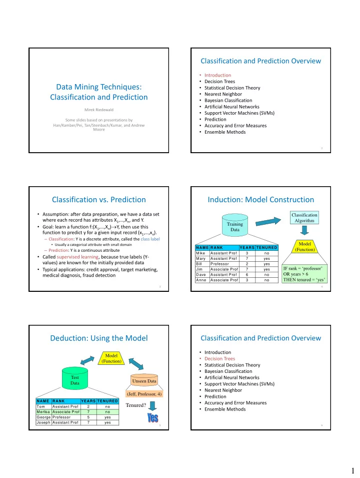
Classification and Prediction Overview • Introduction • Decision Trees Data Mining Techniques: • Statistical Decision Theory • Nearest Neighbor Classification and Prediction • Bayesian Classification • Artificial Neural Networks Mirek Riedewald • Support Vector Machines (SVMs) • Prediction Some slides based on presentations by • Accuracy and Error Measures Han/Kamber/Pei, Tan/Steinbach/Kumar, and Andrew Moore • Ensemble Methods 2 Classification vs. Prediction Induction: Model Construction • Assumption: after data preparation, we have a data set Classification where each record has attributes X 1 ,…, X n , and Y. Algorithm Training • Goal: learn a function f:(X 1 ,…, X n )  Y, then use this Data function to predict y for a given input record (x 1 ,…, x n ). – Classification: Y is a discrete attribute, called the class label Model • Usually a categorical attribute with small domain NAME RANK YEARS TENURED – Prediction: Y is a continuous attribute (Function) Mike Assistant Prof 3 no • Called supervised learning, because true labels (Y- Mary Assistant Prof 7 yes values) are known for the initially provided data Bill Professor 2 yes IF rank = ‘professor’ • Typical applications: credit approval, target marketing, Jim Associate Prof 7 yes OR years > 6 medical diagnosis, fraud detection Dave Assistant Prof 6 no THEN tenured = ‘yes’ Anne Associate Prof 3 no 3 4 Deduction: Using the Model Classification and Prediction Overview • Introduction Model • Decision Trees (Function) • Statistical Decision Theory • Bayesian Classification • Artificial Neural Networks Test Unseen Data Data • Support Vector Machines (SVMs) • Nearest Neighbor (Jeff, Professor, 4) • Prediction NAME RANK YEARS TENURED • Accuracy and Error Measures Tenured? Tom Assistant Prof 2 no • Ensemble Methods Merlisa Associate Prof 7 no George Professor 5 yes Joseph Assistant Prof 7 yes 5 6 1

Example of a Decision Tree Another Example of Decision Tree Single, Splitting Attributes MarSt Tid Refund Marital Taxable Married Divorced Cheat Tid Refund Marital Taxable Status Income Cheat Status Income NO Refund 1 Yes Single 125K No 1 Yes Single 125K No No Refund Yes 2 No Married 100K No 2 No Married 100K No Yes No 3 No Single 70K No 3 No Single 70K No NO TaxInc 4 Yes Married 120K No NO MarSt No < 80K > 80K 4 Yes Married 120K Yes 5 No Divorced 95K Married Single, Divorced 5 No Divorced 95K Yes NO YES 6 No Married 60K No 6 No Married 60K No TaxInc NO 7 Yes Divorced 220K No 7 Yes Divorced 220K No < 80K > 80K 8 No Single 85K Yes 8 No Single 85K Yes 9 No Married 75K No NO YES There could be more than one tree that 9 No Married 75K No 10 No Single 90K Yes fits the same data! 10 No Single 90K Yes 10 10 Model: Decision Tree Training Data 7 8 Apply Model to Test Data Apply Model to Test Data Test Data Test Data Start from the root of tree. Refund Refund Yes No Yes No NO MarSt NO MarSt Married Married Single, Divorced Single, Divorced TaxInc TaxInc NO NO < 80K > 80K < 80K > 80K NO YES NO YES 9 10 Apply Model to Test Data Apply Model to Test Data Test Data Test Data Refund Marital Taxable Refund Marital Taxable Cheat Cheat Status Income Status Income No Married 80K ? No Married 80K ? Refund Refund 10 10 Yes No Yes No NO MarSt NO MarSt Married Married Single, Divorced Single, Divorced TaxInc NO TaxInc NO < 80K > 80K < 80K > 80K NO YES NO YES 11 12 2

Apply Model to Test Data Apply Model to Test Data Test Data Test Data Refund Marital Taxable Refund Marital Taxable Cheat Cheat Status Income Status Income No Married 80K ? No Married 80K ? Refund Refund 10 10 Yes No Yes No NO MarSt NO MarSt Assign Cheat to “No” Married Married Single, Divorced Single, Divorced TaxInc TaxInc NO NO < 80K > 80K < 80K > 80K NO YES NO YES 13 14 Decision Tree Induction Decision Boundary 1 x 2 • Basic greedy algorithm 0.9 X 1 – Top-down, recursive divide-and-conquer < 0.43? 0.8 – At start, all the training records are at the root 0.7 Yes No – Training records partitioned recursively based on split attributes 0.6 X 2 – Split attributes selected based on a heuristic or statistical X 2 0.5 < 0.33? < 0.47? measure (e.g., information gain) 0.4 • Conditions for stopping partitioning Yes No Yes No 0.3 Refund – Pure node (all records belong Yes No 0.2 : 4 : 0 : 0 : 4 to same class) : 0 : 4 : 3 : 0 0.1 – No remaining attributes for NO MarSt 0 further partitioning Married Single, Divorced 0 0.1 0.2 0.3 0.4 0.5 0.6 0.7 0.8 0.9 1 x 1 • Majority voting for classifying the leaf TaxInc NO – No cases left Decision boundary = border between two neighboring regions of different classes. < 80K > 80K For trees that split on a single attribute at a time, the decision boundary is parallel NO YES to the axes. 15 16 Oblique Decision Trees How to Specify Split Condition? • Depends on attribute types – Nominal x + y < 1 – Ordinal – Numeric (continuous) Class = + Class = • Depends on number of ways to split – 2-way split • Test condition may involve multiple attributes – Multi-way split • More expressive representation • Finding optimal test condition is computationally expensive 17 18 3

Splitting Nominal Attributes Splitting Ordinal Attributes • Multi-way split: use as many partitions as • Multi-way split: Size distinct values. Small Large CarType Medium Family Luxury Sports • Binary split: Size Size • Binary split: divides values into two subsets; OR {Small, {Medium, {Large} {Small} Medium} Large} need to find optimal partitioning. • What about this split? CarType CarType Size {Sports, {Family, {Small, OR {Family} {Sports} {Medium} Luxury} Luxury} Large} 19 20 Splitting Continuous Attributes Splitting Continuous Attributes • Different options – Discretization to form an ordinal categorical Taxable Taxable Income Income? attribute > 80K? • Static – discretize once at the beginning < 10K > 80K • Dynamic – ranges found by equal interval bucketing, Yes No equal frequency bucketing (percentiles), or clustering. [10K,25K) [25K,50K) [50K,80K) – Binary Decision: (A < v) or (A  v) (i) Binary split (ii) Multi-way split • Consider all possible splits, choose best one 21 22 How to Determine Best Split How to Determine Best Split • Greedy approach: Before Splitting: 10 records of class 0, 10 records of class 1 – Nodes with homogeneous class distribution are preferred Own Car Student Car? Type? ID? • Need a measure of node impurity: Family Luxury c 1 c 20 Yes No c 10 c 11 Sports C0: 5 C0: 9 C0: 6 C0: 4 C0: 1 C0: 8 C0: 1 C0: 1 C0: 1 C0: 0 C0: 0 ... ... C1: 5 C1: 1 C1: 4 C1: 6 C1: 3 C1: 0 C1: 7 C1: 0 C1: 0 C1: 1 C1: 1 Non-homogeneous, Homogeneous, Which test condition is the best? High degree of impurity Low degree of impurity 23 24 4