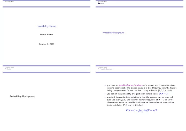
Probability Basics Probability Background Martin Emms October 1, - PowerPoint PPT Presentation

Probability Basics Probability Basics Outline Probability Basics Probability Background Martin Emms October 1, 2020 Probability Basics Probability Basics Outline Probability Background ◮ you have an variable/feature/attribute of a system and it takes on values in some specific set. The classic example is dice throwing, with the feature being the uppermost face of the dice, taking values in { 1 , 2 , 3 , 4 , 5 , 6 } ◮ you talk of the probability of a particular feature value: P ( X = a ) Probability Background ◮ standard frequentist interpretation is that the systems can be observed over and over again, and that the relative frequency of X = a in all the observations tends to a stable fixed value as the number of observations tends to infinity. P ( X = a ) is this limit P ( X = a ) = lim N →∞ freq ( X = a ) / N

Probability Basics Probability Basics Probability Background Probability Background ◮ on this frequentist interpretation you would definitely expect the sum over Independence of two events different outcomes to be 1, so where A is set of possible values for feature X , it is always assumed that ◮ suppose two ’events’ A and B . If the probability of A ∧ B occuring is just � P ( X = a ) = 1 the probability A occuring times the probability of B occuring, you say the a ∈ A events A and B are independent ◮ typically also interested in types or kinds of outcome: not the probability Independence : P ( A ∧ B ) = P ( A ) × P ( B ) of any particular value X = a . Jargon for this is event ◮ Related idea is conditional probability, the probability of A given B : ◮ for example, the ’event’ of dice throw being even can be described as instead of considering how often A occurs, you just consider how often A ( X = 2 ∨ X = 4 ∨ X = 6) occurs in situation which are already B situations. ◮ the relative freq. of (2 or 4 or 6) is by definition the same as the ◮ This is defined to be ( rel . freq 2) + ( rel . freq . 4) + ( rel . freq . 6). So its not surprising that by definition the probability of an ’event’ is the sum of the mutually exclusive Conditional Prob atomic possibilities that are contained within it (ie. ways for it to happen) so P ( A | B ) = P ( A ∧ B ) P ( B ) P ( X = 2 ∨ X = 4 ∨ X = 6) = P ( X = 2) + P ( X = 4) + P ( X = 6) Probability Basics Probability Basics Probability Background Probability Background ◮ there’s a common-sense ’explanation’ for the definition P ( A | B ) = P ( A ∧ B ) ◮ obviously given the definition of P ( A | B ), you have the obvious but as it P ( B ) turns out very useful ◮ you want to take the limit as N tends to infinity of Product Rule N →∞ ( count ( A ∧ B ) in N lim ) P ( A ∧ B ) = P ( A | B ) P ( B ) count ( B ) in N ◮ since P ( A | B ) P ( B ) = P ( B | A ) P ( A ), you also get the famous you get the same thing if you divide top and bottom by N , so Bayesian Inversion N →∞ ( count ( A ∧ B ) in N ( count ( A ∧ B ) in N ) / N lim ) = lim count ( B ) in N ( count ( B ) in N ) / N N →∞ P ( A | B ) = P ( A ∧ B ) = P ( B | A ) P ( A ) lim N →∞ ( count ( A ∧ B ) in N ) / N P ( B ) P ( B ) = lim N →∞ ( count ( B ) in N ) / N P ( A ∧ B ) = P ( B )

Probability Basics Probability Basics Probability Background Probability Background Alternative expressions of independence ◮ Suppose > 1 feature/attribute of your system/situation eg. rolling a red & a green dice. Using X for red & Y for green can specify events with their values and their probs with expressions such as: 1 P ( X = 1 , Y = 2) ◮ recall independence was defined to be P ( A ∧ B ) = P ( A ) × P ( B ). Given and the probability of such an event is called a joint probability the definition of conditional probability there are equivalent formulations ◮ if A is range of values for X & B is range for Y , the must have of independence in terms of conditional probability: � P ( X = a , Y = b ) = 1 Independence : P ( A | B ) = P ( A ) a ∈ A , b ∈ B Independence : P ( B | A ) = P ( B ) ◮ can wish to consider the probs of events specified by the value on just one feature (eg. those where X=1) and the probs. of these are called marginal probabilities and are obtained by summing the joints with all possible NOTE: each of these on its own is equivalent to P ( A ∧ B ) = P ( A ) × P ( B ) values of the other feature � P ( X = 1) = P ( X = 1 , Y = b ) b ∈ B 1 note comma often used instead of ∧ Probability Basics Probability Basics Probability Background Probability Background Chain Rule ◮ the conditional probability function for two features X and Y is ◮ generalising to more variables, you can derive the indispensable P ( X | Y ) = P ( X , Y ) chain rule P ( Y ) so for any pair of values a for X and b for Y , the value of this function is P ( X , Y , Z ) = P ( Z | ( X , Y )) × P ( X , Y ) = P ( Z | ( X , Y )) × P ( Y | X ) × P ( X ) P ( X = a , Y = b ) / P ( Y = b ) ◮ you say P ( X | Y ) = P ( X ) and the features X and Y are independent in P ( X 1 . . . X n ) = P ( X n | ( X 1 . . . X n − 1 )) × . . . × P ( X 2 | X 1 ) × P ( X 1 ) case for every value a for X and b for Y you have P ( X = a , Y = b ) important to note that this chain-rule re-expression of a joint probability = P ( X = a ) P ( Y = b ) as a product does not make any independence assumptions Notation: typically P ( Z | ( X , Y )) is written as P ( Z | X , Y )

Probability Basics Probability Background Conditional Independence ◮ there is a notion of conditional independence. It may be that two variables X and Y are not in general independent, but given a value for a third variable Z , X and Y become independent. Conditional Indpt P ( X , Y | Z ) = P ( X | Z ) P ( Y | Z ) ◮ as with straightforward independence there is an alternative expression for this, stating how a conditioning factor can be dropped Conditional Indpt altern. def P ( X | Y , Z ) = P ( X | Z ) ◮ Real-life cases of this arise where Z describes a cause , which manifests itself into two effects X and Y , which though very dependent on Z , do not directly influence each other ◮ The theories behind Speech Recognition and Machine Translation typically make a lot of conditional independence assumptions