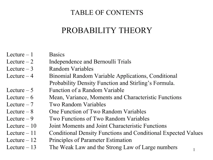

TABLE OF CONTENTS PROBABILITY THEORY Lecture – 1 Basics Lecture – 2 Independence and Bernoulli Trials Lecture – 3 Random Variables Lecture – 4 Binomial Random Variable Applications, Conditional Probability Density Function and Stirling’s Formula. Lecture – 5 Function of a Random Variable Lecture – 6 Mean, Variance, Moments and Characteristic Functions Lecture – 7 Two Random Variables Lecture – 8 One Function of Two Random Variables Lecture – 9 Two Functions of Two Random Variables Lecture – 10 Joint Moments and Joint Characteristic Functions Lecture – 11 Conditional Density Functions and Conditional Expected Values Lecture – 12 Principles of Parameter Estimation Lecture – 13 The Weak Law and the Strong Law of Large numbers 1
STOCHASTIC PROCESSES Lecture – 14 Stochastic Processes - Introduction Lecture – 15 Poisson Processes Lecture – 16 Mean square Estimation Lecture – 17 Long Term Trends and Hurst Phenomena Lecture – 18 Power Spectrum Lecture – 19 Series Representation of Stochastic processes Lecture – 20 Extinction Probability for Queues and Martingales Note: These lecture notes are revised periodically with new materials → and examples added from time to time. Lectures 1 11 are used at Polytechnic for a first level graduate course on “Probability → theory and Random Variables”. Parts of lectures 14 19 are used at Polytechnic for a “Stochastic Processes” course. These notes are intended for unlimited worldwide use. However the user must acknowledge the present website www.mhhe.com/papoulis as the source of information. Any feedback may be addressed to pillai@hora.poly.edu 2 S. UNNIKRISHNA PILLAI
PROBABILITY THEORY 1. Basics Probability theory deals with the study of random phenomena, which under repeated experiments yield different outcomes that have certain underlying patterns about them. The notion of an experiment assumes a set of repeatable conditions that allow any number of identical repetitions. When an experiment is performed under these ξ conditions, certain elementary events occur in different i but completely uncertain ways. We can assign nonnegative ξ number as the probability of the event in various P ξ ( ), i i 3 ways: PILLAI
Laplace’s Classical Definition: The Probability of an event A is defined a-priori without actual experimentation as Number of outcomes favorable to A = P ( A ) , (1-1) Total number of possible outcomes provided all these outcomes are equally likely . Consider a box with n white and m red balls. In this case, there are two elementary outcomes: white ball or red ball. n Probability of “selecting a white ball” = . + n m We can use above classical definition to determine the probability that a given number is divisible by a prime p . 4 PILLAI
If p is a prime number, then every p th number (starting with p ) is divisible by p . Thus among p consecutive integers there is one favorable outcome, and hence 1 { } = P a given number is divisible by a prime p (1-2) p Relative Frequency Definition : The probability of an event A is defined as n = A (1-3) P ( A ) lim n → ∞ n where n A is the number of occurrences of A and n is the total number of trials. We can use the relative frequency definition to derive (1-2) as well. To do this we argue that among the integers p , p � , the numbers are divisible by p . 1, 2, 3, � , , n 2 5 PILLAI
Thus there are n / p such numbers between 1 and n . Hence { } P a given number N is divisible by a prime p 1 . n p / = lim (1-4) = n p →∞ n In a similar manner, it follows that 1 { } = 2 P p divides any given number N (1-5) 2 p and 1 { } = P pq divides any given number N . (1-6) pq The axiomatic approach to probability, due to Kolmogorov, developed through a set of axioms (below) is generally recognized as superior to the above definitions, (1-1) and (1-3), as it provides a solid foundation for complicated 6 applications. PILLAI
ξ The totality of all known a priori , constitutes a set Ω , , i the set of all experimental outcomes. { } Ω = ξ ξ ξ , , � , , � (1-7) 1 2 k Ω has subsets Recall that if A is a subset of A , B , C , � . ξ ∈ ξ ∈ Ω Ω , then A . implies From A and B, we can ∪ ∩ A B , A B , A , B , generate other related subsets etc. { } ∪ = ξ ξ ∈ ξ ∈ A B | A or B { } ∩ = ξ ξ ∈ ξ ∈ A B | A and B and { } = ξ | ξ ∉ A A (1-8) 7 PILLAI
A B A A A B A ∩ A ∪ B B A Fig.1.1 ∩ B = φ A , • If the empty set, then A and B are said to be mutually exclusive (M.E). • A partition of Ω is a collection of mutually exclusive subsets of Ω such that their union is Ω . ∪ ∩ = φ = Ω A A , and A . (1-9) i j i = i 1 A 1 A 2 B A A i A A j n Fig. 1.2 8 ∩ B = φ A PILLAI
De-Morgan’s Laws: ∪ = ∩ ∩ = ∪ (1-10) A B A B ; A B A B A B A B A B B A A ∪ B A ∪ A ∩ B B Fig.1.3 • Often it is meaningful to talk about at least some of the subsets of Ω as events, for which we must have mechanism to compute their probabilities. Example 1.1: Consider the experiment where two coins are simultaneously tossed. The various elementary events are 9 PILLAI
ξ = ξ = ξ = ξ = ( H , H ), ( H , T ), ( T , H ), ( T , T ) 1 2 3 4 and { } . Ω = ξ ξ ξ ξ , , , 1 2 3 4 { } = ξ ξ ξ The subset is the same as “Head A , , 1 2 3 has occurred at least once” and qualifies as an event. Suppose two subsets A and B are both events, then consider = A ∪ “Does an outcome belong to A or B ” B = A ∩ B “Does an outcome belong to A and B ” “Does an outcome fall outside A” ? 10 PILLAI
Thus the sets etc., also qualify as ∪ ∩ A B , A B , A , B , events. We shall formalize this using the notion of a Field. • Field : A collection of subsets of a nonempty set Ω forms a field F if Ω ∈ (i) F ∈ ∈ (1-11) (ii) If A F , then A F ∈ ∈ ∪ ∈ (iii) If A F and B F , then A B F . Using (i) - (iii), it is easy to show that etc., ∩ ∩ A B , A B , also belong to F . For example, from (ii) we have ∈ ∈ and using (iii) this gives ∪ ∈ A F , B F , A B F ; applying (ii) again we get where we ∪ = ∩ ∈ A B A B F , have used De Morgan’s theorem in (1-10). 11 PILLAI
∈ ∈ Thus if then A F , B F , { } . = Ω ∪ ∩ ∪ F , A , B , A , B , A B , A B , A B , � (1-12) From here on wards, we shall reserve the term ‘event’ only to members of F . = ξ Assuming that the probability of elementary p P ( ) i i outcomes of Ω are apriori defined, how does one ξ i assign probabilities to more ‘complicated’ events such as A , B , AB , etc., above? The three axioms of probability defined below can be used to achieve that goal. 12 PILLAI
Axioms of Probability For any event A, we assign a number P ( A ), called the probability of the event A . This number satisfies the following three conditions that act the axioms of probability. ≥ (i) P ( A ) 0 (Probabili ty is a nonnegativ e number) Ω = (ii) P ( ) 1 (Probabili ty of the whole set is unity) (1-13) ∩ = φ ∪ = + (iii) If A B , then P ( A B ) P ( A ) P ( B ). (Note that (iii) states that if A and B are mutually exclusive (M.E.) events, the probability of their union is the sum of their probabilities.) 13 PILLAI
The following conclusions follow from these axioms: ∪ A = Ω a. Since we have using (ii) A , ∪ = Ω = P( A A ) P ( ) 1 . ∩ A ∈ φ But and using (iii), A , ∪ = + = = − (1-14) P( A A ) P ( A ) P( A ) 1 or P( A ) 1 P ( A ). { } { } . ∩ φ = φ b. Similarly, for any A, A ( { } ) ∪ φ = + φ Hence it follows that P A P ( A ) P ( ) . { } { } ∪ φ = φ = But and thus A A , P 0 . (1-15) c. Suppose A and B are not mutually exclusive (M.E.)? How does one compute ∪ B = P ( A ) ? 14 PILLAI
To compute the above probability, we should re-express A ∪ in terms of M.E. sets so that we can make use of B the probability axioms. From Fig.1.4 we have A A B ∪ = ∪ A B A A B , (1-16) where A and are clearly M.E. events. A B A ∪ B Thus using axiom (1-13-iii) Fig.1.4 ∪ = ∪ = + P ( A B ) P ( A A B ) P ( A ) P ( A B ). (1-17) To compute we can express B as P ( B A ), = ∩ Ω = ∩ ∪ B B B ( A A ) = ∩ ∪ ∩ = ∪ (1-18) ( B A ) ( B A ) BA B A Thus (1-19) = + P ( B ) P ( BA ) P ( B A ), since and are M.E. events. BA = = AB B A A B 15 PILLAI
Recommend
More recommend