Chapter 3: Basics from Probability Theory and Statistics 3.1 - PowerPoint PPT Presentation

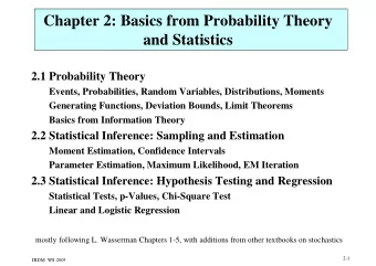
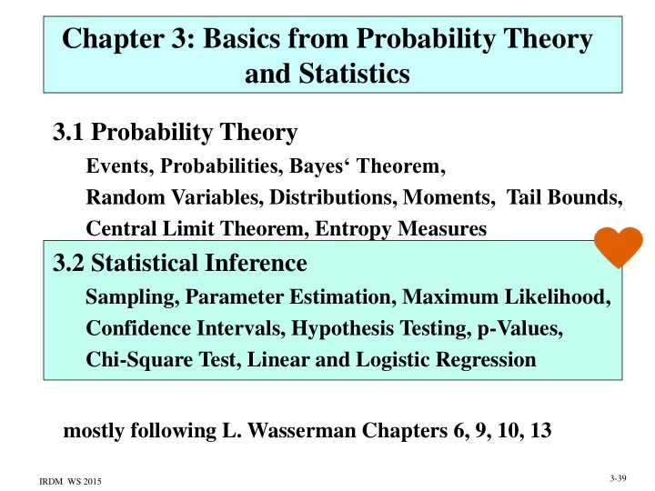
Chapter 3: Basics from Probability Theory and Statistics 3.1 Probability Theory Events, Probabilities, Bayes‘ Theorem, Random Variables, Distributions, Moments, Tail Bounds, Central Limit Theorem, Entropy Measures 3.2 Statistical Inference Sampling, Parameter Estimation, Maximum Likelihood, Confidence Intervals, Hypothesis Testing, p-Values, Chi-Square Test, Linear and Logistic Regression mostly following L. Wasserman Chapters 6, 9, 10, 13 3-39 IRDM WS 2015

3.2 Statistical Inference A statistical model is a set of distributions (or regression functions), e.g., all unimodal, smooth distributions. A parametric model is a set that is completely described by a finite number of parameters, (e.g., the family of Normal distributions). Statistical inference : given a sample X 1 , ..., X n how do we infer the distribution or its parameters within a given model. For multivariate models with one specific „ outcome (response )“ variable Y , this is called prediction or regression, for discrete outcome variable also classification . r(x) = E[Y | X=x] is called the regression function . Example for classification: biomedical markers  cancer or not Example for regression: business indicators  stock price 3-40 IRDM WS 2015

Sampling Illustrated Distribution X Samples (population of interest) X 1 , X 2 , …, X n Statistical Inference: What can we say about X based on X 1 , X 2 , …, X n ? Example: estimate the average salary in Germany? Approach 1: ask your 10 neighbors Approach 2: ask 100 random people you spot on the Internet Approach 2: ask all 1000 living Germans in Wikipedia Approach 4: ask 1000 random people from all age groups, jobs , … 3-41 IRDM WS 2015

Basic Types of Statistical Inference Given: independent and identically distributed (iid) samples X 1 , X 2 , …, X n from (unknown) distribution X • Parameter estimation: What is the parameter p of a Bernoulli coin? What are the values of  and  of a Normal distribution? What are  1 ,  2 ,  1 ,  2 of a Poisson mixture? • Confidence intervals: What is the interval [mean  tolerance] s.t. the expectation of my observations or measurements falls into the interval with high confidence? • Hypothesis testing: H 0 : p=1/2 (fair coin) vs. H 1 : p  1/2 H0: p1 = p2 (methods have same precision) vs. H1: p1  p2 • Regression (for parameter fitting) 3-42 IRDM WS 2015

3.2.1 Statistical Parameter Estimation A point estimator for a parameter  of a prob. distribution is a random variable X derived from a random sample X 1 , ..., X n . Examples: n 1   Sample mean: X : X i n  i 1 n 1 2 2  i   Sample variance: S : ( X X )  n 1  i 1 An estimator T for parameter  is unbiased   E [ T ] if ;   otherwise the estimator has bias . E [ T ] An estimator on a sample of size n is consistent        if lim n P [ T ] 1 for each 0   Sample mean and sample variance are unbiased, consistent estimators with minimal variance. 3-43 IRDM WS 2015

Estimation Error Let = T(  ) be an estimator for parameter  over sample X 1 , ..., X n . ˆ  n ˆ  The distribution of is called the sampling distribution. n ˆ 𝑡𝑓 𝑊𝑏𝑠(  𝜄 = 𝜄 𝑜 ) The standard error for is: n ˆ  The mean squared error (MSE) for is: n ˆ ˆ 2      MSE( ) E[( ) ] n ˆ ˆ 2     bias ( ) Var[ ] n n If bias  0 and se  0 then the estimator is consistent. ˆ  The estimator is asymptotically Normal if n ˆ    ( )/ se converges in distribution to standard Normal N(0,1) n 3-44 IRDM WS 2015

Nonparametric Estimation ˆ The empirical distribution function is the cdf that F n 1 ˆ  n   puts prob. mass 1/n at each data point X i : F ( x ) I( X x )  n i i 1 n where indicator function I( 𝑌 𝑗 ≤ 𝑦) is 1 if 𝑌 𝑗 ≤ 𝑦 and 0 otherwise A statistical functional T(F) is any function of F, e.g., mean, variance, skewness, median, quantiles, correlation ˆ ˆ The plug-in estimator of  = T(F) is: n   T( F ) n 3-45 IRDM WS 2015

Nonparametric Estimation: Histograms Instead of the full empirical distribution, often compact data synopses may be used, such as histograms where X 1 , ..., X n are grouped into m cells (buckets or bins) c 1 , ..., c m with bucket boundaries lb(c i ) and ub(c i ) s.t. lb(c 1 ) =  , ub(c m ) =  , ub(c i ) = lb(c i+1 ) for 1  i<m, and 1  ˆ n    freq(c i ) = F ( x ) I(lb( c ) X ub( c ))    n i i 1 n Histograms provide a (discontinuous) density estimator . Example: X 1 = X 2 = 1 X 3 = X 4 = X 5 = 2 X 6 = … X 10 = 3 X 11 = … X 14 = 4 X 15 = … X 17 = 5 X 18 = X 19 = 6 X 20 = 7 3-46 IRDM WS 2015

Different Kinds of Histograms equidistant buckets Sources: en.wikipedia.org de.wikipedia.org non-equidistant buckets 3-47 IRDM WS 2015

Method of Moments • Suppose parameter θ = ( θ 1 , …, θ k ) has k components • Compute j -th moment for 1 ≤ j ≤ k : • Compute j -th sample moment for 1 ≤ j ≤ k : • Method-of-moments estimate of θ is obtained by solving a system of k equations in k unknowns: Method-of-moments estimators are usually consistent and asympotically Normal, but may be biased 3-48 IRDM WS 2015

Example: Method of Moments Let X 1 , …, X n ~ Normal(  ,  2 ) 𝛽 1 = 𝐹 𝜄 𝑌 = 𝜈 𝛽 2 = 𝐹 𝜄 𝑌 2 = 𝑊𝑏𝑠 𝑌 + 𝐹 𝑌 2 = 𝜏 2 + 𝜈 2 Solve the equation system: 𝑜 𝑜 𝛽 1 = 1 𝛽 2 = 1 𝜏 2 + 𝜈 2 = 𝛽 2 = 𝜈 = 𝛽 1 = 𝑜 𝑌 𝑗 2 𝑜 𝑌 𝑗 𝑗=1 𝑗=1 𝑜 𝑜 𝜈 = 1 𝜏 2 = 1 Solution: 𝑌 𝑗 − 𝑜 𝑌 𝑗 = 𝑌 2 𝑜 𝑌 𝑗=1 𝑗=1 3-49 IRDM WS 2015

Parametric Inference: Maximum Likelihood Estimators (MLE) Estimate parameter  of a postulated distribution f(  ,x) such that the probability that the data of the sample are generated by this distribution is maximized.  Maximum likelihood estimation: Maximize L(x 1 ,...,x n ,  ) = P[x 1 , ..., x n originate from f(  ,x)] often written as 𝜾 𝑵𝑴𝑭 = 𝒃𝒔𝒉𝒏𝒃𝒚 𝜾 L(  , x 1 ,...,x n ) 𝒐 = 𝒃𝒔𝒉𝒏𝒃𝒚 𝜾 𝒋=𝟐 𝒈(𝒚 𝒋 , , 𝜾) or maximize log L if analytically untractable  use numerical iteration methods 3-50 IRDM WS 2015

MLE Properties Maximum Likelihood Estimators are consistent, asymptotically Normal, and asymptotically optimal in the following sense: Consider two estimators U and T which are asymptotically Normal. Let u 2 and t 2 denote the variances of the two Normal distributions to which U and T converge in probability. The asymptotic relative efficiency of U to T is ARE(U,T) = t 2 /u 2 . ˆ   Theorem: For an MLE and any other estimator n n the following inequality holds: ˆ    ARE( , ) 1 n n 3-51 IRDM WS 2015

Simple Example for Maximum Likelihood Estimator given: • coin with Bernoulli distribution with unknown parameter p für head, 1-p for tail • sample (data): k times head with n coin tosses needed: maximum likelihood estimation of p Let L(k, n, p) = P[sample is generated from distr. with param. p]   n  k n k     p ( 1 p )   k Maximize log-likelihood function log L (k, n, p):   n      log L log k logp (n k) log (1 p)     k   k log L k n k  p     0 n   p p 1 p 3-52 IRDM WS 2015

Advanced Example for Maximum Likelihood Estimator given: • Poisson distribution with parameter  (expectation) • sample (data): numbers x 1 , ..., x n  N 0 needed: maximum likelihood estimation of  Let r be the largest among these numbers, and let f 0 , ..., f r be the absolute frequencies of numbers 0, ..., r. f i   i  r        L ( x ,..., x , ) e   1 n i !    i 0 r  i f i  n r   1 ln L i  ˆ      i 0         x x f 1 0 i i      r n    i 1 i 0 f i  i 0 3-53 IRDM WS 2015

Sophisticated Example for Maximum Likelihood Estimator given: • discrete uniform distribution over [1,  ]  N 0 and density f(x) = 1/  • sample (data): numbers x 1 , ..., x n  N 0 MLE for  is max{x 1 , ..., x n } (see Wasserman p. 124) 3-54 IRDM WS 2015

MLE for Parameters of Normal Distributions 2   ( x ) i n    n 1 2  2       2 L ( x ,..., x , , ) e   1 n     2  i 1   n ln( L) 1      2( x ) 0 i   2 i 1  2   n ln( L ) n 1 2        ( x ) 0 i 2 2 4      2 2 i 1 n n 1 1  2 2  ˆ   ˆ    ˆ   x ( x ) i i n n   i 1 i 1 3-55 IRDM WS 2015