Outline 1. Bayes Law L7: Probability Basics 2. Probability - PDF document

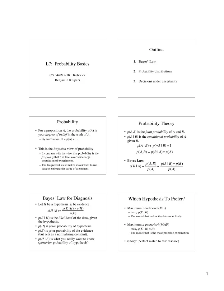
Outline 1. Bayes’ Law L7: Probability Basics 2. Probability distributions CS 344R/393R: Robotics Benjamin Kuipers 3. Decisions under uncertainty Probability Probability Theory • For a proposition A , the probability p ( A ) is • p ( A,B ) is the joint probability of A and B . your degree of belief in the truth of A . • p ( A | B ) is the conditional probability of A – By convention, 0 ≤ p(A) ≤ 1. given B . p ( A | B ) + p ( ¬ A | B ) = 1 • This is the Bayesian view of probability. p ( A , B ) = p ( B | A ) � p ( A ) – It contrasts with the view that probability is the frequency that A is true, over some large population of experiments. • Bayes Law : p ( B | A ) = p ( A , B ) p ( A ) = p ( A | B ) � p ( B ) – The frequentist view makes it awkward to use data to estimate the value of a constant. p ( A ) Bayes’ Law for Diagnosis Which Hypothesis To Prefer? • Let H be a hypothesis, E be evidence. • Maximum Likelihood (ML) p ( H | E ) = p ( E | H ) � p ( H ) – max H p ( E | H ) p ( E ) – The model that makes the data most likely • p ( E | H ) is the likelihood of the data, given the hypothesis. • Maximum a posteriori (MAP) • p ( H ) is prior probability of hypothesis. – max H p ( E | H ) p ( H ) • p ( E ) is prior probability of the evidence – The model that is the most probable explanation (but acts as a normalizing constant). • p ( H | E ) is what you really want to know • (Story: perfect match to rare disease) ( posterior probability of hypothesis). 1

Independence Bayes Law • Two random variables are independent if • The denominator in Bayes Law acts as a – p ( X,Y ) = p ( X ) p ( Y ) normalizing constant: – p ( X | Y ) = p ( X ) p ( H | E ) = p ( E | H ) p ( H ) – p ( Y | X ) = p ( Y ) = � p ( E | H ) p ( H ) p ( E ) – These are all equivalent. 1 � = p ( E ) � 1 = • X and Y are conditionally independent given Z if � p ( E | H ) p ( H ) – p ( X,Y | Z ) = p ( X | Z ) p ( Y | Z ) H – p ( X | Y, Z ) = p ( X | Z ) – p ( Y | X, Z ) = p ( Y | Z ) • It ensures that the probabilities sum to 1 • Independence simplifies inference. across all the hypotheses H . Accumulating Evidence (Naïve Bayes) Bayes Nets Represent Dependence p ( H | d 1 , d 2 L d n ) = p ( H ) p ( d 1 | H ) p ( d 2 | H ) p ( d 2 ) L p ( d n | H ) • The nodes are random variables. p ( d 1 ) p ( d n ) • The links represent dependence. p ( X i | parents ( X i )) n p ( d i | H ) p ( H | d 1 , d 2 L d n ) = p ( H )* � – Independence can be inferred from network p ( d i ) i = 1 • The network represents how the joint n probability distribution can be decomposed. � p ( H | d 1 , d 2 L d n ) = � p ( H )* p ( d i | H ) n � p ( X 1 , L X n ) = p ( X i | parents ( X i )) i = 1 n i = 1 � log p ( H | d 1 , d 2 L d n ) = log p ( H ) + log p ( d i | H ) + � � • There are effective propagation algorithms. i = 1 Simple Bayes Net Example Outline 1. Bayes’ Law 2. Probability distributions 3. Decisions under uncertainty 2

Expectations Variance and Covariance • Let x be a random variable. • The variance is E [ ( x - E [ x ]) 2 ] • The expected value E [ x ] is the mean: N 2 ] = 1 2 = E [( x � x � 2 N ) ( x i � x ) � � x = 1 � � N E [ x ] = x p ( x ) dx x i 1 N 1 • Covariance matrix is E [ ( x - E [ x ])( x - E [ x ]) T ] – The probability-weighted mean of all possible N C ij = 1 values. The sample mean approaches it. � ( x ik � x i )( x jk � x j ) N • Expected value of a vector x is by component. k = 1 T E [ x ] = x = [ x 1 , L x n ] – Divide by N − 1 to make the sample variance an unbiased estimator for the population variance. Biased and Unbiased Estimators Covariance Matrix • Strictly speaking, the sample variance • Along the diagonal, C ii are variances. N 2 ] = 1 2 = E [( x � x � 2 ) ( x i � x ) � • Off-diagonal C ij are essentially correlations. N 1 is a biased estimate of the population � � 2 C 1,1 = � 1 C 1,2 C 1, N variance. An unbiased estimator is: N � � 1 s 2 = � ) 2 ( x i � x 2 C 2,1 C 2,2 = � 2 � � N � 1 1 • But : “If the difference between N and N − 1 � � O M ever matters to you, then you are probably � � 2 L C N ,1 C N , N = � N up to no good anyway …” [Press, et al] � � Independent Variation Dependent Variation • x and y are • c and d are random Gaussian random variables. variables ( N =100) • Generated with • Generated with c=x+y d=x-y σ x =1 σ y =3 • Covariance matrix: • Covariance matrix: C cd = 10.62 � � 7.93 � C xy = 0.90 � 0.44 � � � � � � 7.93 8.84 � � 0.44 8.82 � � 3

Gaussian (Normal) Distribution Estimates and Uncertainty • Completely described by N ( µ , σ ) • Conditional probability density function – Mean µ – Standard deviation σ , variance σ 2 � ( x � µ ) 2 / 2 � 2 1 2 � e � Illustrating the Central Limit Thm The Central Limit Theorem – Add 1, 2, 3, 4 variables from the same distribution. • The sum of many random variables – with the same mean, but – with arbitrary conditional density functions, converges to a Gaussian density function. • If a model omits many small unmodeled effects, then the resulting error should converge to a Gaussian density function. Detecting Modeling Error Outline • Every model is incomplete. – If the omitted factors are all small, the 1. Bayes’ Law resulting errors should add up to a Gaussian. 2. Probability distributions • If the error between a model and the data is not Gaussian, – Then some omitted factor is not small. 3. Decisions under uncertainty – One should find the dominant source of error and add it to the model. 4

Tests: Sensor Noise and Diagnostic Errors and Decision Thresholds Sensor Interpretation • Interpreting sensor values is like diagnosis. • Overlapping response Test=Pos Test=Neg to different cases: Disease True False No Yes present Positive Negative hit miss Disease False True false correct alarm reject absent Positive Negative • Every test has false positives and negatives. – Sonar( fwd )= d implies Obstacle-at-distance( d ) ?? ROC The Test d ' = separation Curves Threshold spread Requires a • The overlap Trade-Off d ′ controls the trade-off between • You can’t types of eliminate all errors. error. • For more, search on • Choose which Signal Detection errors are Theory . important Bayesian Reasoning • One strength of Bayesian methods is that they reason with probability distributions, not just the most likely individual case. • For more, see Andrew Moore’s tutorial slides – http://www.autonlab.org/tutorials/ • Coming up: – Regression to find models from data – Kalman filters to track dynamical systems – Visual object trackers. 5