Alex Psomas: Lecture 14. Probability Basics Review Probability is - PowerPoint PPT Presentation

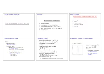
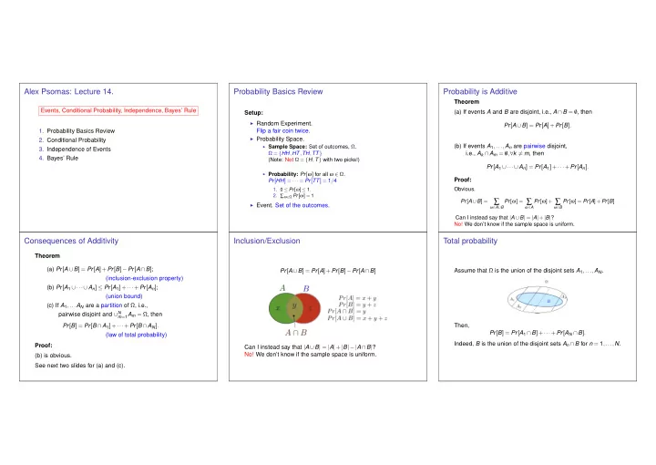
Alex Psomas: Lecture 14. Probability Basics Review Probability is Additive Theorem Events, Conditional Probability, Independence, Bayes’ Rule (a) If events A and B are disjoint, i.e., A ∩ B = / 0 , then Setup: ◮ Random Experiment. Pr [ A ∪ B ] = Pr [ A ]+ Pr [ B ] . 1. Probability Basics Review Flip a fair coin twice. ◮ Probability Space. 2. Conditional Probability (b) If events A 1 ,..., A n are pairwise disjoint, ◮ Sample Space: Set of outcomes, Ω . 3. Independence of Events Ω = { HH , HT , TH , TT } i.e., A k ∩ A m = / 0 , ∀ k � = m , then 4. Bayes’ Rule (Note: Not Ω = { H , T } with two picks!) Pr [ A 1 ∪···∪ A n ] = Pr [ A 1 ]+ ··· + Pr [ A n ] . ◮ Probability: Pr [ ω ] for all ω ∈ Ω . Proof: Pr [ HH ] = ··· = Pr [ TT ] = 1 / 4 Obvious. 1. 0 ≤ Pr [ ω ] ≤ 1 . 2. ∑ ω ∈ Ω Pr [ ω ] = 1 . Pr [ A ∪ B ] = ∑ Pr [ ω ] = ∑ Pr [ ω ]+ ∑ Pr [ ω ] = Pr [ A ]+ Pr [ B ] ◮ Event. Set of the outcomes. ω ∈ A ∪ B ω ∈ A ω ∈ B Can I instead say that | A ∪ B | = | A | + | B | ? No! We don’t know if the sample space is uniform. Consequences of Additivity Inclusion/Exclusion Total probability Theorem (a) Pr [ A ∪ B ] = Pr [ A ]+ Pr [ B ] − Pr [ A ∩ B ] ; Pr [ A ∪ B ] = Pr [ A ]+ Pr [ B ] − Pr [ A ∩ B ] Assume that Ω is the union of the disjoint sets A 1 ,..., A N . (inclusion-exclusion property) (b) Pr [ A 1 ∪···∪ A n ] ≤ Pr [ A 1 ]+ ··· + Pr [ A n ] ; (union bound) (c) If A 1 ,... A N are a partition of Ω , i.e., pairwise disjoint and ∪ N m = 1 A m = Ω , then Pr [ B ] = Pr [ B ∩ A 1 ]+ ··· + Pr [ B ∩ A N ] . Then, Pr [ B ] = Pr [ A 1 ∩ B ]+ ··· + Pr [ A N ∩ B ] . (law of total probability) Indeed, B is the union of the disjoint sets A n ∩ B for n = 1 ,..., N . Proof: Can I instead say that | A ∪ B | = | A | + | B |−| A ∩ B | ? No! We don’t know if the sample space is uniform. (b) is obvious. See next two slides for (a) and (c).

Roll a Red and a Blue Die. Conditional probability: example. A similar example. Two coin flips (fair coin). First flip is heads. Probability of two Two coin flips(fair coin). At least one of the flips is heads. heads? → Probability of two heads? Ω = { HH , HT , TH , TT } ; Uniform probability space. Ω = { HH , HT , TH , TT } ; uniform. Event A = first flip is heads: A = { HH , HT } . Event A = at least one flip is heads. A = { HH , HT , TH } . New sample space: A ; uniform still. New sample space: A ; uniform still. E 1 = ‘Red die shows 6’ ; E 2 = ‘Blue die shows 6’ Event B = two heads. Event B = two heads. E 1 ∪ E 2 = ‘At least one die shows 6’ The probability of two heads if the first flip is heads. The probability of two heads if at least one flip is heads. Pr [ E 1 ] = 6 36 , Pr [ E 2 ] = 6 36 , Pr [ E 1 ∪ E 2 ] = 11 The probability of B given A is 1 / 3. 36 . The probability of B given A is 1 / 2. Conditional Probability: A non-uniform example Another non-uniform example Yet another non-uniform example Consider Ω = { 1 , 2 ,..., N } with Pr [ n ] = p n . Consider Ω = { 1 , 2 ,..., N } with Pr [ n ] = p n . Let A = { 2 , 3 , 4 } , B = { 1 , 2 , 3 } . Let A = { 3 , 4 } , B = { 1 , 2 , 3 } . Ω P r [ ω ] 3/10 Red Green 4/10 Yellow 2/10 Blue 1/10 Physical experiment Probability model Ω = { Red, Green, Yellow, Blue } Pr [ Red | Red or Green ] = 3 7 = Pr [ Red ∩ (Red or Green) ] p 3 = Pr [ A ∩ B ] Pr [ A | B ] = . p 2 + p 3 = Pr [ A ∩ B ] Pr [ Red or Green ] Pr [ A | B ] = . p 1 + p 2 + p 3 Pr [ B ] p 1 + p 2 + p 3 Pr [ B ]

Conditional Probability. More fun with conditional probability. Yet more fun with conditional probability. Toss a red and a blue die, sum is 7, Toss a red and a blue die, sum is 4, what is probability that red is 1? What is probability that red is 1? Definition: The conditional probability of B given A is Pr [ B | A ] = Pr [ A ∩ B ] Pr [ A ] A ∩ B In A ! A A B B In B ? Must be in A ∩ B . Pr [ B | A ] = Pr [ A ∩ B ] Pr [ A ] . Pr [ B | A ] = | B ∩ A | = 1 3 ; versus Pr [ B ] = 1 / 6. Pr [ B | A ] = | B ∩ A | = 1 6 ; versus Pr [ B ] = 1 | A | 6 . | A | B is more likely given A . Observing A does not change your mind about the likelihood of B . Emptiness.. Gambler’s fallacy. Product Rule Suppose I toss 3 balls into 3 bins. A =“1st bin empty”; B =“2nd bin empty.” What is Pr [ A | B ] ? Recall the definition: Flip a fair coin 51 times. A = “first 50 flips are heads” Pr [ B | A ] = Pr [ A ∩ B ] . B = “the 51st is heads” Pr [ A ] Pr [ B | A ] ? Hence, A = { HH ··· HT , HH ··· HH } Pr [ A ∩ B ] = Pr [ A ] Pr [ B | A ] . B ∩ A = { HH ··· HH } Consequently, Uniform probability space. Pr [ B | A ] = | B ∩ A | = 1 2 . Pr [ B ] = Pr [ { ( a , b , c ) | a , b , c ∈ { 1 , 3 } ] = Pr [ { 1 , 3 } 3 ] = 8 Pr [ A ∩ B ∩ C ] = Pr [( A ∩ B ) ∩ C ] | A | 27 = Pr [ A ∩ B ] Pr [ C | A ∩ B ] Same as Pr [ B ] . Pr [ A ∩ B ] = Pr [( 3 , 3 , 3 )] = 1 27 = Pr [ A ] Pr [ B | A ] Pr [ C | A ∩ B ] . The likelihood of 51st heads does not depend on the previous flips. Pr [ A | B ] = Pr [ A ∩ B ] = ( 1 / 27 ) ( 8 / 27 ) = 1 / 8 ; vs. Pr [ A ] = 8 27 . Pr [ B ] A is less likely given B : If second bin is empty the first is more likely to have balls in it.

Product Rule Correlation Correlation Event A : the person has lung cancer. Event B : the person is a heavy smoker. Pr [ A | B ] = 1 . 17 × Pr [ A ] . Theorem Product Rule An example. Let A 1 , A 2 ,..., A n be events. Then Random experiment: Pick a person at random. A second look. Event A : the person has lung cancer. Pr [ A 1 ∩···∩ A n ] = Pr [ A 1 ] Pr [ A 2 | A 1 ] ··· Pr [ A n | A 1 ∩···∩ A n − 1 ] . Event B : the person is a heavy smoker. Note that Proof: By induction. Pr [ A ∩ B ] Assume the result is true for n . (It holds for n = 2.) Then, Pr [ A | B ] = 1 . 17 × Pr [ A ] ⇔ = 1 . 17 × Pr [ A ] Pr [ A | B ] = 1 . 17 × Pr [ A ] . Pr [ B ] Pr [ A 1 ∩···∩ A n ∩ A n + 1 ] ⇔ Pr [ A ∩ B ] = 1 . 17 × Pr [ A ] Pr [ B ] Conclusion: = Pr [ A 1 ∩···∩ A n ] Pr [ A n + 1 | A 1 ∩···∩ A n ] ⇔ Pr [ B | A ] = 1 . 17 × Pr [ B ] . ◮ Smoking increases the probability of lung cancer by 17 % . = Pr [ A 1 ] Pr [ A 2 | A 1 ] ··· Pr [ A n | A 1 ∩···∩ A n − 1 ] Pr [ A n + 1 | A 1 ∩···∩ A n ] , ◮ Smoking causes lung cancer. Conclusion: so that the result holds for n + 1. ◮ Lung cancer increases the probability of smoking by 17 % . ◮ Lung cancer causes smoking. Really? Causality vs. Correlation Proving Causality Total probability Events A and B are positively correlated if Assume that Ω is the union of the disjoint sets A 1 ,..., A N . Pr [ A ∩ B ] > Pr [ A ] Pr [ B ] . Proving causality is generally difficult. One has to eliminate (E.g., smoking and lung cancer.) external causes of correlation and be able to test the cause/effect relationship (e.g., randomized clinical trials). A and B being positively correlated does not mean that A Some difficulties: causes B or that B causes A . ◮ A and B may be positively correlated because they have a Other examples: common cause. (E.g., being a rabbit.) Then, Pr [ B ] = Pr [ A 1 ∩ B ]+ ··· + Pr [ A N ∩ B ] . ◮ Tesla owners are more likely to be rich. That does not ◮ If B precedes A , then B is more likely to be the cause. mean that poor people should buy a Tesla to get rich. (E.g., smoking.) However, they could have a common Indeed, B is the union of the disjoint sets A n ∩ B for n = 1 ,..., N . cause that induces B before A . (E.g., smart, CS70, Tesla.) ◮ People who go to the opera are more likely to have a good Thus, career. That does not mean that going to the opera will Pr [ B ] = Pr [ A 1 ] Pr [ B | A 1 ]+ ··· + Pr [ A N ] Pr [ B | A N ] . improve your career. ◮ Rabbits eat more carrots and do not wear glasses. Are carrots good for eyesight?