CS70: Alex Psomas: Lecture 19. 1. Random Variables: Brief Review 2. - PowerPoint PPT Presentation
CS70: Alex Psomas: Lecture 19. 1. Random Variables: Brief Review 2. Some details on distributions: Geometric. Poisson. 3. Joint distributions. 4. Linearity of Expectation. Random Variables: Definitions Is a random variable random? NO! Is a
CS70: Alex Psomas: Lecture 19. 1. Random Variables: Brief Review 2. Some details on distributions: Geometric. Poisson. 3. Joint distributions. 4. Linearity of Expectation.
Random Variables: Definitions Is a random variable random? NO! Is a random variable a variable? NO! Great name!
Random Variables: Definitions Definition A random variable, X , for a random experiment with sample space Ω is a function X : Ω → ℜ . Thus, X ( · ) assigns a real number X ( ω ) to each ω ∈ Ω . Definitions (a) For a ∈ ℜ , one defines X − 1 ( a ) := { ω ∈ Ω | X ( ω ) = a } . (b) For A ⊂ ℜ , one defines X − 1 ( A ) := { ω ∈ Ω | X ( ω ) ∈ A } . (c) The probability that X = a is defined as Pr [ X = a ] = Pr [ X − 1 ( a )] . (d) The probability that X ∈ A is defined as Pr [ X ∈ A ] = Pr [ X − 1 ( A )] . (e) The distribution of a random variable X , is { ( a , Pr [ X = a ]) : a ∈ A } , where A is the range of X . That is, A = { X ( ω ) , ω ∈ Ω } .
Expectation - Definition Definition: The expected value (or mean, or expectation) of a random variable X is E [ X ] = ∑ a × Pr [ X = a ] . a ∈ R Theorem: E [ X ] = ∑ X ( ω ) × Pr [ ω ] . ω ∈ Ω
An Example Flip a fair coin three times. Ω = { HHH , HHT , HTH , THH , HTT , THT , TTH , TTT } . X = number of H ’s: { 3 , 2 , 2 , 2 , 1 , 1 , 1 , 0 } . ◮ Range of X ? { 0 , 1 , 2 , 3 } . All the values X can take. ◮ X − 1 ( 2 ) ? X − 1 ( 2 ) = { HHT , HTH , THH } . All the outcomes ω such that X ( ω ) = 2. ◮ Is X − 1 ( 1 ) an event? YES . It’s a subset of the outcomes. ◮ Pr [ X ] ? This doesn’t make any sense bro.... ◮ Pr [ X = 2 ] ? Pr [ X = 2 ] = Pr [ X − 1 ( 2 )] = Pr [ { HHT , HTH , THH } ] = Pr [ { HHT } ]+ Pr [ { HTH } ]+ Pr [ { THH } ] = 3 8
An Example Flip a fair coin three times. Ω = { HHH , HHT , HTH , THH , HTT , THT , TTH , TTT } . X = number of H ’s: { 3 , 2 , 2 , 2 , 1 , 1 , 1 , 0 } . Thus, X ( ω ) Pr [ ω ] = 3 8 + 2 8 + 2 8 + 2 8 + 1 8 + 1 8 + 1 8 + 0 = 12 E [ X ] = ∑ 8 ω ∈ Ω Also, a × Pr [ X = a ] = 3 × 1 8 + 2 × 3 8 + 1 × 3 8 + 0 × 1 E [ X ] = ∑ 8 . a ∈ R
Win or Lose. Expected winnings for heads/tails games, with 3 flips? Recall the definition of the random variable X : { HHH , HHT , HTH , HTT , THH , THT , TTH , TTT } → { 3 , 1 , 1 , − 1 , 1 , − 1 , − 1 , − 3 } . E [ X ] = 3 × 1 8 + 1 × 3 8 − 1 × 3 8 − 3 × 1 8 = 0 . Can you ever win 0? Apparently: expected value is not a common value, by any means. It doesn’t have to be in the range of X . The expected value of X is not the value that you expect! Great name once again! It is the average value per experiment, if you perform the experiment many times: X 1 + ··· + X n , when n ≫ 1 . n The fact that this average converges to E [ X ] is a theorem: the Law of Large Numbers. (See later.)
Geometric Distribution Let’s flip a coin with Pr [ H ] = p until we get H . For instance: ω 1 = H , or ω 2 = T H , or ω 3 = T T H , or ω n = T T T T ··· T H . Note that Ω = { ω n , n = 1 , 2 ,... } . (Notice: no distribution yet!) Let X be the number of flips until the first H . Then, X ( ω n ) = n . Also, Pr [ X = n ] = ( 1 − p ) n − 1 p , n ≥ 1 .
Geometric Distribution Pr [ X = n ] = ( 1 − p ) n − 1 p , n ≥ 1 .
Geometric Distribution: A weird trick Recall the Geometric Distribution. Pr [ X = n ] = ( 1 − p ) n − 1 p , n ≥ 1 . Note that ∞ ∞ ∞ ∞ ( 1 − p ) n − 1 = p ( 1 − p ) n − 1 p = p ( 1 − p ) n . ∑ ∑ ∑ ∑ Pr [ X = n ] = n = 1 n = 1 n = 1 n = 0 n = 0 a n for | a | < 1. S = We want to analyze S := ∑ ∞ 1 1 − a . Indeed, 1 + a + a 2 + a 3 + ··· S = a + a 2 + a 3 + a 4 + ··· aS = 1 + a − a + a 2 − a 2 + ··· = 1 . ( 1 − a ) S = Hence, ∞ 1 ∑ Pr [ X = n ] = p 1 − ( 1 − p ) = 1 . n = 1
Geometric Distribution: Expectation X = D G ( p ) , i.e., Pr [ X = n ] = ( 1 − p ) n − 1 p , n ≥ 1 . One has ∞ ∞ n ( 1 − p ) n − 1 p . ∑ ∑ E [ X ] = nPr [ X = n ] = n = 1 n = 1 Thus, p + 2 ( 1 − p ) p + 3 ( 1 − p ) 2 p + 4 ( 1 − p ) 3 p + ··· E [ X ] = ( 1 − p ) p + 2 ( 1 − p ) 2 p + 3 ( 1 − p ) 3 p + ··· ( 1 − p ) E [ X ] = p + ( 1 − p ) p + ( 1 − p ) 2 p + ( 1 − p ) 3 p + ··· pE [ X ] = by subtracting the previous two identities ∞ ( 1 − p ) n = 1 . ∑ = p n = 0 Hence, E [ X ] = 1 p .
Geometric Distribution: Memoryless I flip a coin (probability of H is p ) until I get H . What’s the probability that I flip it exactly 100 times? ( 1 − p ) 99 p What’s the probability that I flip it exactly 100 times if (given that) the first 20 were T ? Same as flipping it exactly 80 times! ( 1 − p ) 79 p .
Geometric Distribution: Memoryless Let X be G ( p ) . Then, for n ≥ 0, Pr [ X > n ] = Pr [ first n flips are T ] = ( 1 − p ) n . Theorem Pr [ X > n + m | X > n ] = Pr [ X > m ] , m , n ≥ 0 . Proof: Pr [ X > n + m and X > n ] Pr [ X > n + m | X > n ] = Pr [ X > n ] Pr [ X > n + m ] = Pr [ X > n ] ( 1 − p ) n + m = ( 1 − p ) m = ( 1 − p ) n = Pr [ X > m ] .
Geometric Distribution: Memoryless - Interpretation Pr [ X > n + m | X > n ] = Pr [ X > m ] , m , n ≥ 0 . Pr [ X > n + m | X > n ] = Pr [ A | B ] = Pr [ A ] = Pr [ X > m ] . The coin is memoryless, therefore, so is X .
Geometric Distribution: Yet another look Theorem: For a r.v. X that takes the values { 0 , 1 , 2 ,... } , one has ∞ ∑ E [ X ] = Pr [ X ≥ i ] . i = 1 [See later for a proof.] If X = G ( p ) , then Pr [ X ≥ i ] = Pr [ X > i − 1 ] = ( 1 − p ) i − 1 . Hence, ∞ ∞ 1 − ( 1 − p ) = 1 1 ( 1 − p ) i − 1 = ( 1 − p ) i = ∑ ∑ E [ X ] = p . i = 1 i = 0
Expected Value of Integer RV Theorem: For a r.v. X that takes values in { 0 , 1 , 2 ,... } , one has ∞ ∑ E [ X ] = Pr [ X ≥ i ] . i = 1 Proof: One has ∞ ∑ E [ X ] = i × Pr [ X = i ] i = 1 ∞ ∑ = i ( Pr [ X ≥ i ] − Pr [ X ≥ i + 1 ]) i = 1 ∞ ∑ = ( i × Pr [ X ≥ i ] − i × Pr [ X ≥ i + 1 ]) i = 1 ∞ ∑ = ( i × Pr [ X ≥ i ] − ( i − 1 ) × Pr [ X ≥ i ]) i = 1 ∞ ∑ = Pr [ X ≥ i ] . i = 1
Poisson Distribution: Definition and Mean Definition Poisson Distribution with parameter λ > 0 X = P ( λ ) ⇔ Pr [ X = m ] = λ m m ! e − λ , m ≥ 0 . Fact: E [ X ] = λ . Proof: ∞ ∞ m × λ m λ m m ! e − λ = e − λ ∑ ∑ E [ X ] = ( m − 1 )! m = 1 m = 1 ∞ λ m + 1 ∞ λ m e − λ = e − λ λ ∑ ∑ = m ! m ! m = 0 m = 0 e − λ λ e λ = λ . = Used Taylor expansion of e x at 0 : e x = ∑ ∞ x n n ! . n = 0
Simeon Poisson The Poisson distribution is named after:
Indicators Definition Let A be an event. The random variable X defined by � 1 , if ω ∈ A X ( ω ) = 0 , if ω / ∈ A is called the indicator of the event A . Note that Pr [ X = 1 ] = Pr [ A ] and Pr [ X = 0 ] = 1 − Pr [ A ] . Hence, E [ X ] = 1 × Pr [ X = 1 ]+ 0 × Pr [ X = 0 ] = Pr [ A ] . This random variable X ( ω ) is sometimes written as 1 { ω ∈ A } or 1 A ( ω ) . Thus, we will write X = 1 A .
Review: Distributions ◮ U [ 1 ,..., n ] : Pr [ X = m ] = 1 n , m = 1 ,..., n ; E [ X ] = n + 1 2 ; � n p m ( 1 − p ) n − m , m = 0 ,..., n ; ◮ B ( n , p ) : Pr [ X = m ] = � m E [ X ] = np ; (TODO) ◮ G ( p ) : Pr [ X = n ] = ( 1 − p ) n − 1 p , n = 1 , 2 ,... ; E [ X ] = 1 p ; ◮ P ( λ ) : Pr [ X = n ] = λ n n ! e − λ , n ≥ 0; E [ X ] = λ .
Joint distribution. Two random variables, X and Y , in prob space: (Ω , P ( · )) . What is ∑ x Pr [ X = x ] ? 1. What ∑ x Pr [ Y = y ] ? 1. Let’s think about: Pr [ X = x , Y = y ] . What is ∑ x , y Pr [ X = x , Y = y ] ? Are the events “ X = x , Y = y ” disjoint? Yes! Y and X are functions on Ω Do they cover the entire sample space? Yes! X and Y are functions on Ω . So, ∑ x , y Pr [ X = x , Y = y ] = 1. Joint Distribution: Pr [ X = x , Y = y ] . Marginal Distributions: Pr [ X = x ] and Pr [ Y = y ] . Important for inference.
Two random variables, same outcome space. Experiment: pick a random person. X = number of episodes of Games of Thrones they have seen. Y = number of episodes of Westworld they have seen. X = 0 1 2 3 5 40 All Pr 0.3 0.05 0.05 0.05 0.05 0.1 0.4 Is this a distribution? Yes! All the probabilities are non-negative and add up to 1. Y = 0 1 5 10 Pr 0.3 0.1 0.1 0.5
Joint distribution: Example. The joint distribution of X and Y is: Y/X 0 1 2 3 5 40 All 0 0.15 0 0 0 0 0.1 0.05 =0.3 1 0 0.05 0.05 0 0 0 0 =0.1 5 0 0 0 0.05 0.05 0 0 =0.1 10 0.15 0 0 0 0 0 0.35 =0.5 =0.3 =0.05 =0.05 =0.05 =0.05 =0.1 =0.4 Is this a valid distribution? Yes! Notice that Pr [ X = a ] and Pr [ Y = b ] are (marginal) distributions! But now we have more information! For example, if I tell you someone watched 5 episodes of Westworld, they definitely didn’t watch all the episodes of GoT.
Combining Random Variables Definition Let X , Y , Z be random variables on Ω and g : ℜ 3 → ℜ a function. Then g ( X , Y , Z ) is the random variable that assigns the value g ( X ( ω ) , Y ( ω ) , Z ( ω )) to ω . Thus, if V = g ( X , Y , Z ) , then V ( ω ) := g ( X ( ω ) , Y ( ω ) , Z ( ω )) . Examples: ◮ X k ◮ ( X − a ) 2 ◮ a + bX + cX 2 +( Y − Z ) 2 ◮ ( X − Y ) 2 ◮ X cos ( 2 π Y + Z ) .
Recommend
More recommend
Explore More Topics
Stay informed with curated content and fresh updates.

