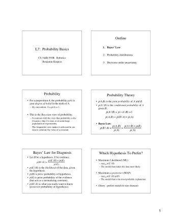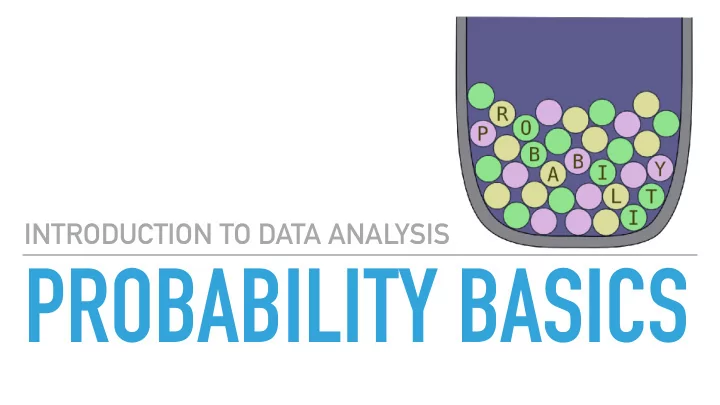
PROBABILITY BASICS INTRODUCTION TO DATA ANALYSIS LEARNING GOALS - PowerPoint PPT Presentation

INTRODUCTION TO DATA ANALYSIS PROBABILITY BASICS

INTRODUCTION TO DATA ANALYSIS LEARNING GOALS ▸ become familiar with the notion of probability ▸ axiomatic definition & interpretation ▸ joint, marginal & conditional probability ▸ Bayes rule ▸ random variables ▸ probability distributions in R ▸ probability distributions as approximated by samples

Probability

INTRODUCTION TO DATA ANALYSIS ELEMENTARY OUTCOMES AND EVENTS ▸ a random process has elementary outcomes Ω = { ω 1 , ω 2 , …} ▸ elementary outcomes are mutually exclusive exhausts the space of possibilities ▸ Ω ▸ any is an event A ⊆ Ω ▸ standard set-theoretic notation for negation, conjunction, disjunction etc. ▸ example “rolling an odd number”

INTRODUCTION TO DATA ANALYSIS PROBABILITY DISTRIBUTION

INTRODUCTION TO DATA ANALYSIS INTERPRETATIONS OF PROBABILITY ▸ Frequentist: probabilities are generalizations of intuitions/facts about frequencies of events in repeated executions of a random event. ▸ Subjectivist: probabilities are subjective beliefs by a rational agent who is uncertain about the outcome of a random event. ▸ Realist: probabilities are a property of an intrinsically random world.

INTRODUCTION TO DATA ANALYSIS

INTRODUCTION TO DATA ANALYSIS PROBABILITY DISTRIBUTIONS AS SAMPLES ▸ No matter our preferred metaphysical interpretation, we can approximate a probability distribution by either: I can you a ▸ a large set of representative samples; or sample give! ▸ an oracle that returns a sample if needed.

Structured events

INTRODUCTION TO DATA ANALYSIS

INTRODUCTION TO DATA ANALYSIS JOINT PROBABILITY DISTRIBUTIONS ▸ Structured elementary outcomes: Ω flip − & − draw = Ω flip × Ω draw ▸ shorthand notation P ( heads , black ) instead of P ( ⟨ heads , black ⟩ )

INTRODUCTION TO DATA ANALYSIS MARGINAL DISTRIBUTIONS ▸ if and , the marginal probability of is: Ω = Ω 1 × … Ω n A i ⊆ Ω i A i ∑ P ( A i ) = P ( A 1 , …, A i − 1 , A i , A i +1 , … A n ) A 1 ⊆Ω 1 ,…, A i − 1 ⊆Ω i − 1 , A i +1 ⊆Ω i +1 ,…, A n ⊆Ω n ∑ P ( black ) = 0.3 P ( white ) = 0.7 ∑ P ( heads ) = 0.5 P ( tails ) = 0.5

Conditional probability & Bayes rule

INTRODUCTION TO DATA ANALYSIS CONDITIONAL PROBABILITY P ( A ∣ B ) = P ( A ∩ B ) ▸ the conditional probability of A given B is: P ( B ) P ( black ∣ heads ) = P ( black , heads ) = 0.1 0.5 = 0.2 P ( heads ) ∑ P ( black ) = 0.3 P ( white ) = 0.7 ∑ P ( heads ) = 0.5 P ( tails ) = 0.5

INTRODUCTION TO DATA ANALYSIS BAYES RULE ▸ Bayes rule follows straightforwardly from the definition of conditional P ( A ∣ B ) = P ( A ∩ B ) probability: P ( B ) P ( A ∩ B ) = P ( B ∣ A ) P ( A ) P ( B ∣ A ) = P ( A ∣ B ) P ( B ) P ( A ) P ( B ∩ A ) = P ( A ∣ B ) ⋅ P ( B )

INTRODUCTION TO DATA ANALYSIS P ( B ∣ A ) = P ( A ∣ B ) P ( B ) PREVIEW ::: BAYES RULE FOR DATA ANALYSIS P ( A ) likelihood of data prior over parameters P ( θ ∣ D ) = P ( D ∣ θ ) P ( θ ) P ( D ) posterior over parameters marginal likelihood of data

Random variables

INTRODUCTION TO DATA ANALYSIS RANDOM VARIABLES ▸ a random variable is a function: X : Ω → ℝ ▸ if range of is countable, we speak of a discrete random variable X ▸ otherwise, we speak of a continuous random variable ▸ think: distribution of a summary statistic ▸ notation: ▸ shorthand notation instead of P ({ ω ∈ Ω ∣ X ( ω ) = 2}) P ( X = x ) ▸ similarly write stuff like or P ( X ≤ x ) P (1 ≤ X ≤ 2)

INTRODUCTION TO DATA ANALYSIS RANDOM VARIABLE ::: EXAMPLES

INTRODUCTION TO DATA ANALYSIS CUMULATIVE DISTRIBUTION & PROBABILITY MASS ::: DISCRETE RV S Binom ( K = k ; n , θ ) = ( k ) θ k (1 − θ ) n − k n probability mass function

INTRODUCTION TO DATA ANALYSIS CUMULATIVE DISTRIBUTION & PROBABILITY MASS ::: DISCRETE RV S Binom ( K = k ; n , θ ) = ( k ) θ k (1 − θ ) n − k n cumulative probability function

INTRODUCTION TO DATA ANALYSIS CUMULATIVE DISTRIBUTION & PROBABILITY MASS ::: CONTINUOUS RV S exp ( − ( x − μ ) 2 ) 1 𝒪 ( X = x ; μ , σ ) = 2 σ 2 2 σ 2 π probability density function

INTRODUCTION TO DATA ANALYSIS CUMULATIVE DISTRIBUTION & PROBABILITY MASS ::: CONTINUOUS RV S exp ( − ( x − μ ) 2 ) 1 𝒪 ( X = x ; μ , σ ) = 2 σ 2 2 σ 2 π cumulative probability function

INTRODUCTION TO DATA ANALYSIS EXPECTED VALUE OF A RANDOM VARIABLE ▸ the expected value of random variable is: X : Ω → ℝ 𝔽 X = ∑ if is discreet: X x f X ( x ) x 𝔽 X = ∫ x f X ( x ) d x if is continuous: X ‣ think: mean of a representative sample of X

INTRODUCTION TO DATA ANALYSIS VARIANCE OF A RANDOM VARIABLE ▸ the variance of random variable is: X : Ω → ℝ Var ( X ) = ∑ ( 𝔽 X − x ) 2 f X ( x ) if is discreet: X x Var ( X ) = ∫ ( 𝔽 X − x ) 2 f X ( x ) d x if is continuous: X ‣ think: variance of a representative sample of X

INTRODUCTION TO DATA ANALYSIS COMPOSITE RANDOM VARIABLES ▸ we can compose random variables with standard mathematical operations e.g., , where and are random variables Z = X + Y X Y ▸ easy to conceive of this in terms of samples

Probability distributions in R

INTRODUCTION TO DATA ANALYSIS PROBABILITY DISTRIBUTIONS IN R ▸ for each distribution mydist , there are four types of functions ▸ dmydist(x, ...) density function gives the (mass/density) for x f ( x ) ▸ pmydist(x, ...) cumulative probability function gives cumulative distribution for x F ( x ) ▸ qmydist(p, ...) quantile function gives value x with p = pmydist(x, ...) ▸ rmydist(n, ...) random sample function returns n samples from the distribution

INTRODUCTION TO DATA ANALYSIS EXAMPLE ::: NORMAL DISTRIBUTION