Today CS 188: Artificial Intelligence Uncertainty Spring 2006 - PDF document

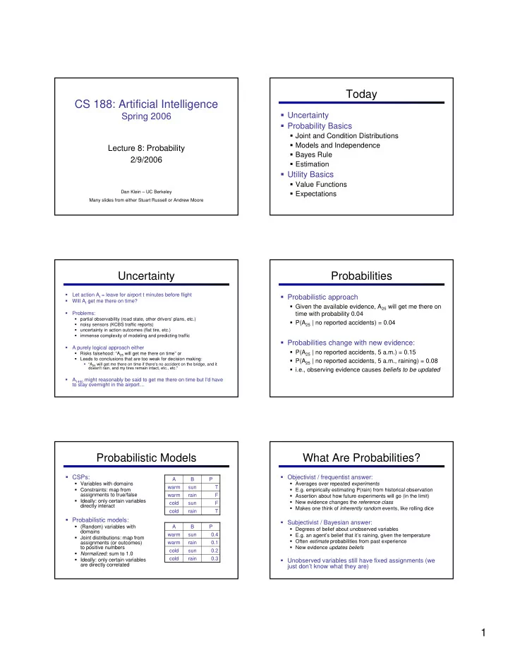
Today CS 188: Artificial Intelligence � Uncertainty Spring 2006 � Probability Basics � Joint and Condition Distributions � Models and Independence Lecture 8: Probability � Bayes Rule 2/9/2006 � Estimation � Utility Basics � Value Functions � Expectations Dan Klein – UC Berkeley Many slides from either Stuart Russell or Andrew Moore Uncertainty Probabilities � Let action A t = leave for airport t minutes before flight � Probabilistic approach � Will A t get me there on time? � Given the available evidence, A 25 will get me there on � Problems: time with probability 0.04 � partial observability (road state, other drivers' plans, etc.) � P(A 25 | no reported accidents) = 0.04 � noisy sensors (KCBS traffic reports) � uncertainty in action outcomes (flat tire, etc.) � immense complexity of modeling and predicting traffic � Probabilities change with new evidence: � A purely logical approach either � P(A 25 | no reported accidents, 5 a.m.) = 0.15 � Risks falsehood: “A 25 will get me there on time” or � Leads to conclusions that are too weak for decision making: � P(A 25 | no reported accidents, 5 a.m., raining) = 0.08 � “A 25 will get me there on time if there's no accident on the bridge, and it doesn't rain, and my tires remain intact, etc., etc.'' � i.e., observing evidence causes beliefs to be updated � A 1440 might reasonably be said to get me there on time but I'd have to stay overnight in the airport… Probabilistic Models What Are Probabilities? � CSPs: � Objectivist / frequentist answer: A B P � Variables with domains � Averages over repeated experiments warm sun T � Constraints: map from � E.g. empirically estimating P(rain) from historical observation assignments to true/false warm rain F � Assertion about how future experiments will go (in the limit) � Ideally: only certain variables � New evidence changes the reference class cold sun F directly interact � Makes one think of inherently random events, like rolling dice cold rain T � Probabilistic models: � Subjectivist / Bayesian answer: � (Random) variables with A B P � Degrees of belief about unobserved variables domains � E.g. an agent’s belief that it’s raining, given the temperature warm sun 0.4 � Joint distributions: map from � Often estimate probabilities from past experience assignments (or outcomes) warm rain 0.1 � New evidence updates beliefs to positive numbers cold sun 0.2 � Normalized: sum to 1.0 cold rain 0.3 � Ideally: only certain variables � Unobserved variables still have fixed assignments (we are directly correlated just don’t know what they are) 1

Probabilities Everywhere? Distributions on Random Vars � � Not just for games of chance! A joint distribution over a set of random variables: � I’m snuffling: am I sick? is a map from assignments (or outcome , or atomic event ) to reals: � Email contains “FREE!”: is it spam? � Tooth hurts: have cavity? � Safe to cross street? � 60 min enough to get to the airport? � Robot rotated wheel three times, how far did it advance? � Size of distribution if n variables with domain sizes d? � Why can a random variable have uncertainty? � Must obey: � Inherently random process (dice, etc) � Insufficient or weak evidence � Unmodeled variables � Ignorance of underlying processes � The world’s just noisy! � Compare to fuzzy logic , which has degrees of truth , or soft � For all but the smallest distributions, impractical to write out assignments Examples Marginalization � An event is a set E of assignments (or � Marginalization (or summing out) is projecting a joint T S P outcomes) warm sun 0.4 distribution to a sub-distribution over subset of variables warm rain 0.1 cold sun 0.2 cold rain 0.3 � From a joint distribution, we can calculate the probability of any event T P warm 0.5 � T S P Probability that it’s warm AND sunny? cold 0.5 warm sun 0.4 warm rain 0.1 � Probability that it’s warm? cold sun 0.2 S P cold rain 0.3 sun 0.6 � Probability that it’s warm OR sunny? rain 0.4 Conditional Probabilities Conditioning � � Conditioning is fixing some variables and renormalizing Conditional or posterior probabilities: � E.g., P( cavity | toothache ) = 0.8 over the rest: � Given that toothache is all I know… � Notation for conditional distributions: � P( cavity | toothache ) = a single number � P(Cavity, Toothache) = 4-element vector summing to 1 � P(Cavity | Toothache) = Two 2-element vectors, each summing to 1 � If we know more: � P( cavity | toothache , catch ) = 0.9 � P( cavity | toothache , cavity ) = 1 T S P � Note: the less specific belief remains valid after more evidence arrives, but warm sun 0.4 is not always useful T P T P warm rain 0.1 warm 0.1 warm 0.25 � New evidence may be irrelevant, allowing simplification: cold sun 0.2 Normalize Select � P( cavity | toothache, traffic ) = P( cavity | toothache ) = 0.8 cold 0.3 cold 0.75 cold rain 0.3 � This kind of inference, sanctioned by domain knowledge, is crucial 2

Inference by Enumeration Inference by Enumeration � General case: � P(R)? � Evidence variables: S T R P � Query variables: summer warm sun 0.30 � All variables Hidden variables: summer warm rain 0.05 � We want: summer cold sun 0.10 � P(R|winter)? summer cold rain 0.05 � The required summation of joint entries is done by summing out H: winter warm sun 0.10 winter warm rain 0.05 winter cold sun 0.15 � P(R|winter,warm)? � Then renormalizing winter cold rain 0.20 � Obvious problems: � Worst-case time complexity O(d n ) � Space complexity O(d n ) to store the joint distribution The Chain Rule I Lewis Carroll's Sack Problem � Sack contains a red or blue ball, 50/50 � Sometimes joint P(X,Y) is easy to get � We add a red ball � Sometimes easier to get conditional P(X|Y) � If we draw a red ball, what’s the chance of drawing a second red ball? � Variables: � F={r,b} is the original ball � D={r,b} is the ball we draw � Example: P(Sun,Dry)? � Query: P(F=r|D=r) D S P D S P F D P F D P wet sun 0.1 wet sun 0.08 F P r r 1.0 r r R P dry sun 0.9 dry sun 0.72 r 0.5 r b 0.0 r b sun 0.8 wet rain 0.7 wet rain 0.14 b 0.5 b r 0.5 b r rain 0.2 dry rain 0.3 dry rain 0.06 b b 0.5 b b Lewis Carroll's Sack Problem Independence � Two variables are independent if: � Now we have P(F,D) � Want P(F|D=r) � This says that their joint distribution factors into a product two simpler distributions F D P � Independence is a modeling assumption r r 0.5 � Empirical joint distributions: at best “close” to independent r b 0.0 � What could we assume for {Sun, Dry, Toothache, Cavity}? b r 0.25 b b 0.25 � How many parameters in the full joint model? � How many parameters in the independent model? � Independence is like something from CSPs: what? 3

Example: Independence Example: Independence? � Arbitrary joint � N fair, independent coins: distributions can be (poorly) modeled by T P S P independent factors warm 0.5 sun 0.6 H 0.5 H 0.5 H 0.5 cold 0.5 rain 0.4 T 0.5 T 0.5 T 0.5 T S P T S P warm sun 0.4 warm sun 0.3 warm rain 0.1 warm rain 0.2 cold sun 0.2 cold sun 0.3 cold rain 0.3 cold rain 0.2 Conditional Independence Conditional Independence � P(Toothache,Cavity,Catch) has 2 3 = 8 entries (7 independent � Unconditional independence is very rare (two reasons: entries) why?) � If I have a cavity, the probability that the probe catches in it doesn't � Conditional independence is our most basic and robust depend on whether I have a toothache: form of knowledge about uncertain environments: � P(catch | toothache, cavity) = P(catch | cavity) � The same independence holds if I haven't got a cavity: P(catch | toothache, ¬ cavity) = P(catch| ¬ cavity) � � Catch is conditionally independent of Toothache given Cavity: � � What about this domain: P(Catch | Toothache, Cavity) = P(Catch | Cavity) � Traffic � Equivalent statements: � Umbrella � P(Toothache | Catch , Cavity) = P(Toothache | Cavity) � Raining � P(Toothache, Catch | Cavity) = P(Toothache | Cavity) P(Catch | Cavity) � What about fire, smoke, alarm? The Chain Rule II The Chain Rule III � Can always factor any joint distribution as a product of � Write out full joint distribution using chain rule: incremental conditional distributions � P(Toothache, Catch, Cavity) = P(Toothache | Catch, Cavity) P(Catch, Cavity) = P(Toothache | Catch, Cavity) P(Catch | Cavity) P(Cavity) = P(Toothache | Cavity) P(Catch | Cavity) P(Cavity) � Why? P(Cavity) Cav Graphical model notation: • Each variable is a node � This actually claims nothing… • The parents of a node are the other variables which the � What are the sizes of the tables we supply? decomposed joint conditions on T Cat • MUCH more on this to come! P(Toothache | Cavity) P(Catch | Cavity) 4