Quick Tour of Probability CS246: Mining Massive Datasets Winter - PowerPoint PPT Presentation
Quick Tour of Probability Quick Tour of Probability CS246: Mining Massive Datasets Winter 2013 Anshul Mittal Based on previous versions in Winter 2011 and 2012 Quick Tour of Probability Basic Definitions Sample Space : set of all possible
Quick Tour of Probability Quick Tour of Probability CS246: Mining Massive Datasets Winter 2013 Anshul Mittal Based on previous versions in Winter 2011 and 2012
Quick Tour of Probability Basic Definitions Sample Space Ω : set of all possible outcomes Event Space F : a family of subsets of Ω Probability Measure Function P : F → R with properties: 0 ≤ P ( A ) ≤ 1 ( ∀ A ∈ F ) P (Ω) = 1 P ( A ∪ B ) = P ( A ) + P ( B ) − P ( A ∩ B ) If A i ’s are disjoint, then P ( � i A i ) = � i P ( A i )
Quick Tour of Probability Conditional Probability and Independence For events A,B: P ( A | B ) = P ( A ∩ B ) P ( B ) A, B are independent if P ( A | B ) = P ( A ) or equivalently, P ( A ∩ B ) = P ( A ) P ( B ) Bayes’ rule: P ( A | B ) = P ( B | A ) P ( A ) P ( B )
Quick Tour of Probability Random Variables and Distribution A random variable X is a function X : Ω → R Example: Number of heads in 20 tosses of a coin Cumulative Distribution Function (CDF) F X : R → [ 0 , 1 ] s.t. F X ( x ) = P ( X ≤ x ) Probability Mass Function (pmf): If X is discrete then p X ( x ) = P ( X = x ) Probability Density Function (pdf): If X is continuous, f X ( x ) = dF X ( x ) / dx
Quick Tour of Probability Properties of Distribution Functions CDF: 0 ≤ F X ( x ) ≤ 1 F X is monotonically increasing with lim x →−∞ F X ( x ) = 0 and lim x →∞ F X ( x ) = 1 pmf: 0 ≤ p X ( x ) ≤ 1 � x p X ( x ) = 1 For a set A, p X ( A ) = � x ∈ A p X ( x ) pdf: f X ( x ) > 0 � ∞ −∞ f X ( x ) dx = 1 � x ∈ A f X ( x ) dx = P ( X ∈ A )
Quick Tour of Probability Some Common Random Variables X ∼ Bernoulli ( p )( 0 ≤ p ≤ 1 ) : � p : x = 1 p X ( x ) = 1 − p : x = 0 X ∼ Geometric ( p )( 0 ≤ p ≤ 1 ) : p X ( x ) = p ( 1 − p ) x − 1 X ∼ Uniform ( a , b )( a < b ) : 1 � : a ≤ x ≤ b b − a f X ( x ) = 0 : otherwise X ∼ Normal ( µ, σ 2 : 1 − 1 2 σ 2 ( x − µ ) 2 f X ( x ) = e � ( 2 π ) σ
Quick Tour of Probability Expectation and Variance Assume random variable X has pdf f X ( x ) , and g : R → R . Then � E [ g ( X )] = ∞ g ( x ) f X ( x ) dx −∞ For discrete X , E [ g ( X )] = � X g ( x ) p X ( x ) Properties: For any constant ain R , E [ a ] = a E [ ag ( X )] = aE [ g ( X )] Linearity of expectation: E [ g ( X ) + h ( X )] = E [ g ( X )] + E [ h ( X )] Var [ X ] = E [( X − E [ X ]) 2 ] Var [ aX ] = a 2 Var [ X ]
Quick Tour of Probability Some Useful Inequalities Markov’s Inequality: X random variable, and a > 0. Then: P ( | X | ≥ a ) ≤ E [ | X | ] a Chebyshev’s Inequality: If E [ X ] = µ, Var [ X ] = σ 2 , k > 0, then: P ( | X − µ | ≥ k σ ) < = 1 k 2 Chernoff bound: X 1 , . . . , X n iid random variables, with E [ X i ] = µ, X i ∈ 0 , 1 ( ∀ i ≤ i ≤ n ) . Then: n P ( | 1 � X i − µ | ≥ ǫ ) ≤ 2 exp ( − 2 n ǫ 2 ) n i = 1
Recommend
More recommend
Explore More Topics
Stay informed with curated content and fresh updates.
