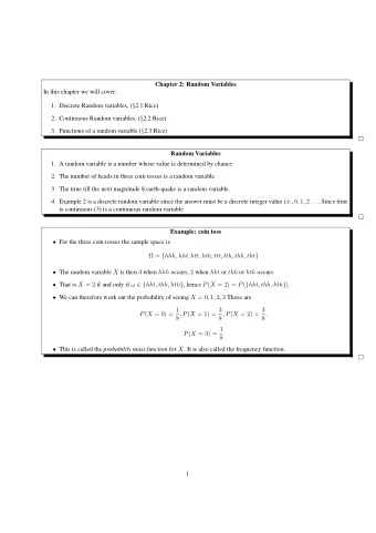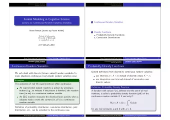
Random Variables Suppose we flip a fair coin twice. What is the - PDF document

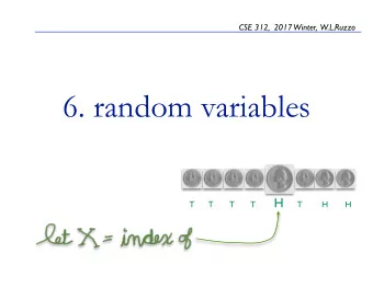
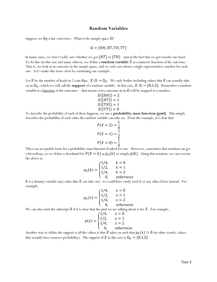
Random Variables Suppose we flip a fair coin twice. What is the sample space Ω ? Ω = {𝐼𝐼, 𝐼𝑈, 𝑈𝐼, 𝑈𝑈} In many cases, we don’t really care whether we got {𝐼𝑈} or {𝑈𝐼} – just in the fact that we got exactly one head. To do this (in this case and many others), we define a random variable 𝑌 as a numeric function of the outcome. That is, we look at an outcome in the sample space, and we only care about a single representative number for each one. Let’s make this more clear by continuing our examp le. Let 𝑌 be the number of heads in 2 coin flips, 𝑌: Ω → Ω 𝑌 . We only bother including values that 𝑌 can actually take on in Ω 𝑌 , which we will call the support of a random variable. In this case, 𝑌: Ω → {0,1,2} . Remember a random variable is a function of the outcomes – that means every outcome 𝜕 in Ω will be mapped to a number. 𝑌({𝐼𝐼}) = 2 𝑌({𝐼𝑈}) = 1 𝑌({𝑈𝐼}) = 1 𝑌({𝑈𝑈}) = 0 To describe the probability of each of these happens, we use a probability mass function (pmf) . This simply describes the probability of each value the random variable can take on. From the example, it’s clear that 𝑄(𝑌 = 2) = 1 4 𝑄(𝑌 = 1) = 1 2 𝑄(𝑌 = 0) = 1 4 This is an acceptable form for a probability mass function if asked for one. However, sometimes this notation can get a bit tedious, so we define a shorthand for 𝑄(𝑌 = 𝑙) as 𝑞 𝑌 (𝑙) or simply 𝑞(𝑙) . Using this notation, we can rewrite the above as 1/4, 𝑙 = 0 1/2, 𝑙 = 1 𝑞 𝑌 (𝑙) = { 1/4, 𝑙 = 2 0, 𝑝𝑢ℎ𝑓𝑠𝑥𝑗𝑡𝑓 𝑙 is a dummy variable (any value that 𝑌 can take on) – we could have easily used 𝑦 or any other letter instead. For example, 1/4, 𝑦 = 0 1/2, 𝑦 = 1 𝑞 𝑌 (𝑦) = { 1/4, 𝑦 = 2 0, 𝑝𝑢ℎ𝑓𝑠𝑥𝑗𝑡𝑓 We can also omit the subscript 𝑌 if it is clear that the pmf we are talking about is for 𝑌 . For example, 1/4, 𝑦 = 0 1/2, 𝑦 = 1 𝑞(𝑦) = { 1/4, 𝑦 = 2 0, 𝑝𝑢ℎ𝑓𝑠𝑥𝑗𝑡𝑓 Another way to define the support is all the values 𝑦 that 𝑌 takes on such that 𝑞 𝑌 (𝑦) > 0 (in other words, values that actually have nonzero probability). The support of 𝑌 in this case is Ω 𝑌 = {0,1,2} . Tsun 1

Sometimes, we are in situations where there are multiple random variables in a question. Say 𝑌 and 𝑍 are random variables, and we write 𝑞(2) . What does this mean? 𝑄(𝑌 = 2) or 𝑄(𝑍 = 2) ? To be clear, we instead write 𝑞 𝑌 (2) = 𝑄(𝑌 = 2) or 𝑞 𝑍 (2) = 𝑄(𝑍 = 2) . It is highly recommended (but not required yet) that you always subscript your probability mass functions. You will have to write subscripts later in this course, so you may as well get used to it now. To summarize, at the beginning we had a full enumeration of the sample space Ω = {𝐼𝐼, 𝐼𝑈, 𝑈𝐼, 𝑈𝑈} 1 with 𝑄({𝐼𝐼}) = 𝑄({𝐼𝑈}) = 𝑄({𝑈𝐼}) = 𝑄({𝑈𝑈}) = 4 . Now, since we only care about how many heads we get, we can instead define the probabilities of the outcomes as 1/4, 𝑙 = 0 1/2, 𝑙 = 1 𝑞 𝑌 (𝑙) = { 1/4, 𝑙 = 2 0, 𝑝𝑢ℎ𝑓𝑠𝑥𝑗𝑡𝑓 The point of random variables is to summarize the outcomes of the sample space in a way that we care. Note that 1 1 1 ∑ 𝑞 𝑌 (𝑙) 4 = 1 , as it should. = 4 + 2 + 𝑙 Functions of Random Variables Consider this contrived example: suppose instead of 𝑌 , we were interested in 𝑌 3 . 𝑌 3 is also a random variable since 𝑌 was a random variable. What does this mean? It literally translates to the cube of 𝑌 , or the cubed number of heads. 𝑌 3 ({𝐼𝐼}) = 8 𝑌 3 ({𝐼𝑈}) = 1 𝑌 3 ({𝑈𝐼}) = 1 𝑌 3 ({𝑈𝑈}) = 0 So we associate {𝐼𝐼} with 2 3 = 8 since it has 2 heads. Notice the other values don’t change since 1 3 = 1 and 0 3 = 0 . Now how do we describe the probability mass function for 𝑌 3 ? 1/4, 𝑙 = 0 1/2, 𝑙 = 1 𝑞 𝑌 3 (𝑙) = { 1/4, 𝑙 = 8 0, 𝑝𝑢ℎ𝑓𝑠𝑥𝑗𝑡𝑓 Notice we don’t touch the probabil ities at all – just the values. Notice that the probabilities do not change so they still sum to 1 . Now, the 𝑌 3 cannot be 2 since there’s no way a cubed number of heads can be 2 . Instead, we reassign the probability to the value 2 3 = 8 . Notice the subscript is especially important in this case as we can distinguish between 𝑞 𝑌 and 𝑞 𝑌 3 . The support is also different - Ω 𝑌 3 = {0,1,8} ≠ {0,1,2} = Ω 𝑌 . Tsun 2

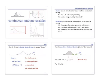
What if two or more values ended up the same? For example, suppose 𝑍 represents the location of a frog starting at the origin who moves one unit either left or right, or not at all. Suppose he has probability of 1/6 of going left or right, and 2/3 of being lazy and not moving. Then 𝑍 has the following pmf: 1/6, 𝑙 = −1 2/3, 𝑙 = 0 𝑞 𝑍 (𝑙) = { 1/6, 𝑙 = 1 0, 𝑝𝑢ℎ𝑓𝑠𝑥𝑗𝑡𝑓 Suppose we are interested only in how far the frog ends up, rather than the exact location. That is, we are interested in 𝑋 = |𝑍| , a new random variable. Then, a trick to find the pmf for 𝑋 is to just directly apply the absolute value function to the values of the pmf. For example: 1/6, 𝑙 = | − 1| 2/3, 𝑙 = |0| 𝑞 𝑋 (𝑙) = { 1/6, 𝑙 = |1| 0, 𝑝𝑢ℎ𝑓𝑠𝑥𝑗𝑡𝑓 Notice that, now |−1| = |1| = 1 . In this case, we simply add the probabilities since they were disjoint to get the final pmf: 2/3, 𝑙 = 0 𝑞 𝑋 (𝑙) = { 1/3, 𝑙 = 1 0, 𝑝𝑢ℎ𝑓𝑠𝑥𝑗𝑡𝑓 1 1 1 This should make sense – think about it. The frog moved one unit away at all with probability 3 , so 6 + 6 = 𝑄(𝑋 = 1) = 𝑞 𝑋 (1) = 1/3 . Other examples of random variables:  The number of heads in 𝑜 independent flips of a fair coin  The number of people who are born every minute  The number of flips of a fair coin until I flip a head  The amount of time I wait until the next bus in minutes  The weight of your backpack in pounds Do you notice something different about the last two examples? They are still random variables, but they can take on an uncountable number of values. I can wait 4.833312 minutes for the next bus, or 𝜌 minutes, or any arbitrary real number. Your backpack could weight 15.3235353 pounds, or 𝑓 5 pounds, or any real number. The first two take on finite values, and the third can take on a countably infinite number of values (the size of the natural numbers). We call a random variable discrete if it takes on a countable number of values. We call a random variable continuous if it takes on an uncountable number of values. The reason we usually write 𝑞 𝑌 (𝑙) instead of 𝑞 𝑌 (𝑦) is because 𝑙 is usually interpreted as an integer, whereas we think of 𝑦 as being any real number. However, either is acceptable. Tsun 3

Expectation Suppose we play the following game: you roll a 10 sided die and I pay you based on what you roll. If you roll a 1 or 3, I will pay you $9 . If you roll an even number, I will pay you $4 . If you roll anything else (5,7,9), I will pay you $6 . Let 𝑌 be the (discrete or continuous?) random variable denoting how much I win from one play of a game. How much do you expect to win in a game? Note that the probability mass function of 𝑌 is 2/10, 𝑙 = 9 5/10, 𝑙 = 4 𝑞 𝑌 (𝑙) = { 3/10, 𝑙 = 6 0, 𝑝𝑢ℎ𝑓𝑠𝑥𝑗𝑡𝑓 2 5 3 And note that ∑ 𝑞 𝑌 (𝑙) 10 = 1 . = 10 + 10 + 𝑙 Maybe it’s too hard to think of how much you expect to win in one game. Since there are 10 outcomes, let’s think of how much we expect to win in 10 games, and then divide that by 10 (why does this make sense?). Let’s play 10 times. Then I expect to win $9 exactly twice (when I roll a 1 or 3), $4 5 times (when I roll an even), and $6 3 times (when I roll 3,5,7,9). Then, my expected winning over 10 games is 9 ∗ 2 + 4 ∗ 5 + 6 ∗ 3 = 56 . Therefore, my expected winning in 1 game is exactly $5.60 . If we had divided by 10 earlier, we could write 10 (9 ∗ 2 + 4 ∗ 5 + 6 ∗ 3) = 9 ∗ 2 1 10 + 4 ∗ 5 10 + 6 ∗ 3 10 = 5.6 This is exactly ∑ 𝑙𝑞 𝑌 (𝑙) ! Notice how we multiplied each possible value of the random variable by its probability. 𝑙 This is the definition of expectation – it is a weighted sum of the outcomes of the random variable, weighted by their probabilities. We define 𝑭[𝒀] = ∑ 𝒍𝒒 𝒀 (𝒍) . 𝒍 Let 𝑌 be how much money I win in my first play of this game, and 𝑍 be how much I win in my second play. Then if 𝑎 = 𝑌 + 𝑍 , 𝑎 would represent the amount of money won in two games. Since 𝑌 and 𝑍 have the same pmf (why?), we expect to win $5.60 in both games – that is 𝐹[𝑌] = 𝐹[𝑍] = 5.6 . Note that we would not say 𝑌 = 𝑍 , since they could take on different values, even though they have the same pmf (and therefore expectation). Something interesting to think about – let 𝑎 = 𝑌 + 𝑍 be the amount of money I win in two plays of this game. Would it make sense that I expect to win 2 ∗ $5.60 = $11.20 ? That is, 𝐹[𝑎] = 𝐹[𝑌 + 𝑍] = 𝐹[𝑌] + 𝐹[𝑍] = 5.6 + 5.6 = 11.2 Yes! This property is called linearity of expectation and will be covered soon. Tsun 4