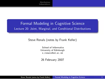
Formal Modeling in Cognitive Science 1 Continuous Random Variables - PowerPoint PPT Presentation

Continuous Random Variables Continuous Random Variables Density Functions Density Functions Formal Modeling in Cognitive Science 1 Continuous Random Variables Lecture 21: Continuous Random Variables; Densities Steve Renals (notes by Frank Keller) 2 Density Functions Probability Density Functions School of Informatics Cumulative Distributions University of Edinburgh s.renals@ed.ac.uk 27 February 2007 Steve Renals (notes by Frank Keller) Formal Modeling in Cognitive Science 1 Steve Renals (notes by Frank Keller) Formal Modeling in Cognitive Science 2 Continuous Random Variables Continuous Random Variables Probability Density Functions Density Functions Density Functions Cumulative Distributions Continuous Random Variables Probability Density Functions Extend definitions from discrete to continuous random variables: We only dealt with discrete (integer-valued) random variables. In use intervals a ≤ X ≤ b instead of discrete values X = x ; many situations, continuous (real-valued) random variables occur. use integration over intervals instead of summation over Examples discrete values. The outcomes of real-life experiments are often continuous: Definition: Probability Density Function An experimental subject reacts to a picture by pressing a button (e.g., to indicate if the picture is familiar): the reaction A function with values f ( x ), defined over the set of all real time (in ms) is a continuous random variable. numbers, is called a probability density function (pdf) of the continuous random variable X if and only if: An EEG machine measures the electrical brain activity when a subjects reads a word: the current (in µ V) is a continuous � b random variable. P ( a ≤ X ≤ b ) = f ( x ) dx a Definition of probability distribution, cumulative distribution, joint for any real constants a and b with a ≤ b . distribution, etc., can be extended to the continuous case. Steve Renals (notes by Frank Keller) Formal Modeling in Cognitive Science 3 Steve Renals (notes by Frank Keller) Formal Modeling in Cognitive Science 4

Continuous Random Variables Probability Density Functions Continuous Random Variables Probability Density Functions Density Functions Cumulative Distributions Density Functions Cumulative Distributions Probability Density Functions Probability Density Functions Plot the function on the previous slide: Example 1 Assume a continuous random variable X with the pdf: � e − x for x > 0 0.8 f ( x ) = 0 elsewhere 0.6 Compute the probability for the interval 0 ≤ X ≤ 1: � b � 1 0.4 � 1 e − x dx = − e − x � P ( a ≤ X ≤ b ) = f ( x ) dx = 0 a 0 ( − e − 1 ) − ( − e 0 ) = − 1 0.2 = e + 1 = 0 . 63 0 0 1 2 3 4 5 x Steve Renals (notes by Frank Keller) Formal Modeling in Cognitive Science 5 Steve Renals (notes by Frank Keller) Formal Modeling in Cognitive Science 6 Continuous Random Variables Probability Density Functions Continuous Random Variables Probability Density Functions Density Functions Cumulative Distributions Density Functions Cumulative Distributions Probability Density Functions Probability Density Functions Theorem: Intervals of pdfs Example If X is a continuous random variable and a and b are real Assume a random variable X with the pdf f ( x ) as follows. Is this a constants with a ≤ b , then: valid pdf? x 2 + 1 1 � for 1 < x ≤ 2 P ( a ≤ X ≤ b ) = P ( a ≤ X < b ) = P ( a < X ≤ b ) = P ( a < X < b ) 2 f ( x ) = 0 elsewhere � ∞ f ( x ) ≥ 0 is true by definition. To show −∞ f ( x ) dx = 1, integrate: Theorem: Valid pdfs � 2 A function can serve as the pdf of a continuous random variable X � ∞ 2 � x 2 + 1 1 2 dx = − 1 x + 1 � f ( x ) dx = 2 x if its values, f ( x ), satisfy the conditions: � � 1 1 −∞ 1 f ( x ) ≥ 0 for each value within its domain; ( − 1 2 + 1 2 · 2) − ( − 1 1 + 1 = 2 · 1) = 1 2 � ∞ −∞ f ( x ) dx = 1. Steve Renals (notes by Frank Keller) Formal Modeling in Cognitive Science 7 Steve Renals (notes by Frank Keller) Formal Modeling in Cognitive Science 8

Continuous Random Variables Probability Density Functions Continuous Random Variables Probability Density Functions Density Functions Cumulative Distributions Density Functions Cumulative Distributions Probability Density Functions Cumulative Distributions Plot the function on the previous slide: In analogy with the discrete case, we can define: 1.6 Definition: Cumulative Distribution If X is a continuous random variable and the value of its 1.2 probability density function at t is f ( t ), then the function given by: � x F ( x ) = P ( X ≤ x ) = f ( t ) dt for − ∞ < x < ∞ 0.8 −∞ is the cumulative distribution of X . 0.4 Intuitively, the cumulative distribution captures the area under the curve defined by f ( t ) from −∞ to x . 0 1 1.2 1.4 1.6 1.8 2 x Steve Renals (notes by Frank Keller) Formal Modeling in Cognitive Science 9 Steve Renals (notes by Frank Keller) Formal Modeling in Cognitive Science 10 Continuous Random Variables Probability Density Functions Continuous Random Variables Probability Density Functions Density Functions Cumulative Distributions Density Functions Cumulative Distributions Cumulative Distributions Cumulative Distributions Example Assume a continuous random variable X with the pdf: Theorem: Value of Cumulative Distribution If f ( x ) and F ( x ) are the values of the pdf and the distribution e − t � for t > 0 f ( t ) = function of X at x , then: 0 elsewhere Integrate for t > 0: P ( a ≤ X ≤ b ) = F ( b ) − F ( a ) � x � x � x for any real constants a and b with a ≤ b and: e − t dt = − e − t � F ( x ) = P ( X ≤ x ) = f ( t ) dt = 0 0 −∞ ( − e − x ) − ( − e 0 ) = − e − x + 1 f ( x ) = dF ( x ) = dx Therefore the cumulative distribution of X is: where the derivative exists. − e − x + 1 � for x > 0 F ( x ) = 0 elsewhere Steve Renals (notes by Frank Keller) Formal Modeling in Cognitive Science 11 Steve Renals (notes by Frank Keller) Formal Modeling in Cognitive Science 12

Continuous Random Variables Probability Density Functions Continuous Random Variables Probability Density Functions Density Functions Cumulative Distributions Density Functions Cumulative Distributions Cumulative Distributions Other Densities Example In analogy with the discrete case, we can define for continuous Use the theorem on the previous slide to compute the probability random variables: P (0 ≤ X ≤ 1) for f ( t ): joint probability density; P (0 ≤ X ≤ 1) = F (1) − F (0) = ( − e − 1 ) − ( − e − 0 ) = − 1 e +1 = 0 . 63 marginal probability density; conditional probability density. Also, verify the derivative of F ( x ): Essentially, we replace the � signs with integrals in the definitions = d ( − e − x ) dF ( x ) for the discrete case. We will not deal with this in detail. = e − x dx dx Steve Renals (notes by Frank Keller) Formal Modeling in Cognitive Science 13 Steve Renals (notes by Frank Keller) Formal Modeling in Cognitive Science 14 Continuous Random Variables Probability Density Functions Density Functions Cumulative Distributions Summary Probability density functions are the probability distributions for continuous random variables; cumulative distributions can also be defined for continuous random variables. Steve Renals (notes by Frank Keller) Formal Modeling in Cognitive Science 15