219323 Probability and Statistics for Software and Knowledge - PowerPoint PPT Presentation

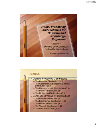
219323 Probability and Statistics for Software and Knowledge Engineers Lecture 2: Random Variables Monchai Sopitkamon, Ph.D.

Outline � Discrete Random Variables (2.1) � Continuous Random Variables (2.2) � Expectation of a Random Variable (2.3) � The Variance of a Random Variable (2.4) � Jointly Distributed Random Variables (2.5) � Functions and Combinations of Random Variables (2.6)

Discrete Random Variables (2.1) � Definition (2.1.1) � Probability Mass Function (2.1.2) � Cumulative Distribution Function (2.1.3)

Discrete Random Variables: Definition I � Random variable: a numerical value assigned to each outcome in the sample space of a certain experiment. � E.g.1, If sample space S = {electrical, mechanical, misuse} containing outcomes (machine breakdown problem) – Each outcome (cause) may be assigned a repair cost (random variable) of $50, $200, and $350, respectively.

Discrete Random Variables: Definition II � E.g.2, Using the 3 power-plant example, suppose the random variable of interest is the number of plants that are generating electricity. Then we get a RV: X = number of plants generating electricity = 0, 1, 2, and 3 (0, 0, 1) (0, 1, 1) (1, 1, 1) (0, 0, 0) (0, 1, 0) (1, 0, 1) (1, 0, 0) �� (1, 1, 0) ��

Discrete Random Variables: Probability Mass Function I (2.1.2) � Pmf. of a random variable X is a set of probability values p i assigned to each of the values x i taken by the discrete RV. � These p i must satisfy 1. 0 ≤ p i ≤ 1 and ∑ = 1 2. . p i i ) = p i → means probability that P ( X = x i RV X takes the value x i is equal to p i

Discrete Random Variables: Probability Mass Function II (2.1.2) � E.g.3, From the machine breakdown problem, suppose – P(cost = $50) = 0.3, – P(cost = $200) = 0.2, and – P(cost = $350) = 0.5 We can summarize the pmf. as: 0.5 Probability $50 $200 $350 x i 0.3 0.2 0.3 0.2 0.5 p i $50 $200 $350 Repair Cost

Discrete Random Variables: Probability Mass Function III (2.1.2) � E.g.4, From e.g.2, – P (no plants are generating electricity) = P (X = 0) = prob. of outcome (0, 0, 0) = 0.07 – P (exactly one plant is generating electricity) = P (X = 1) = P (1, 0, 0) + P (0, 1, 0) + P (0, 0, 1) = 0.04 + 0.03 + 0.16 = 0.23 – P(two plants…) = P (X = 2) …

Discrete Random Variables: Probability Mass Function IV (2.1.2) 0.57 0.23 0.13 0.07 0 1 2 3 0.07 0.23 0.57 0.13 P(X=xi) Number of power plants

Discrete Random Variables: Cumulative Distribution Function (2.1.3) � Cdf of a RV X is the function ∑ P ( X = y ) F ( x ) = P ( X ≤ x ) = y ≤ x F ( x ) = sum of probabilities P ( X = y ) for all y ≤ x F ( x ) is an increasing function – = 1 – lim F ( x ) . x →∞ – Do examples 1 pg. 76 and 4 pg. 77

Outline � Discrete Random Variables (2.1) � Continuous Random Variables (2.2) � Expectation of a Random Variable (2.3) � The Variance of a Random Variable (2.4) � Jointly Distributed Random Variables (2.5) � Functions and Combinations of Random Variables (2.6)

Continuous Random Variables (2.2) � Examples of Continuous Random Variables (2.2.1) � Probability Density Function (2.2.2) � Cumulative Distribution Function (2.2.3)

Continuous Random Variables: Examples of Continuous Random Variables (2.2.1) � Continuous RVs can take any value within a continuous region. � E.g., a RV X that represents the diameter of a randomly selected cylinder made by a company, whose value ranges between 49.5 - 50.5 mm. � E.g., a RV X representing the time to failure of a newly charged battery, whose value is in the interval [0, ∞ ). � E.g., a RV X measuring the actual amount of milk filled in a milk container by a machine, whose value is in the interval [1.95, 2.20] liters.

Continuous Random Variables: Probability Density Function I (2.2.2) � A pdf f ( x ) defines the probabilistic properties of a continuous RV. ∫ = 1 f ( x ) dx � f ( x ) ≥ 0 and statespace b ∫ f ( x ) dx � P ( a ≤ X ≤ b ) = a � Note that the prob. that a continuous RV X takes any certain value a is always 0. Or, mathematically: a ∫ P ( X = a ) = = 0 f ( x ) dx a

Continuous Random Variables: Probability Density Function II (2.2.2) � Difference between discrete and continuous RVs: – Discrete RVs can have nonzero prob. of taking specific values – Continuous RVs have zero prob. of taking specific values, but they can have nonzero prob. of falling within certain continuous regions. – Do examples 14 on pg.83 and 15 on pg.84

Continuous Random Variables: Cumulative Distribution Function I (2.2.3) � The cdf. of a continuous RV X is, similarly to that for a discrete RV, or F ( x ) = P ( X ≤ x ) � F ( x ) is a continuous nondecreasing function starting from 0, at the beginning of state space, and reaching 1, at the end of state space. F ( x ) 1 0 x State space

Continuous Random Variables: Cumulative Distribution Function II (2.2.3) � We can compute cdf. F ( x ) from the pdf. f ( x ) as follows: x ∫ f ( y ) dy F ( x ) = P ( X ≤ x ) = −∞ f ( x ) = dF ( x ) Thus, dx And the prob. that a RV lies within a certain region is: P ( a ≤ X ≤ b ) = P ( X ≤ b ) − P ( X ≤ a ) = F ( b ) − F ( a ) � Do example 14 on pg.87

Outline � Discrete Random Variables (2.1) � Continuous Random Variables (2.2) � Expectation of a Random Variable (2.3) � The Variance of a Random Variable (2.4) � Jointly Distributed Random Variables (2.5) � Functions and Combinations of Random Variables (2.6)

Expectation of a Random Variable (2.3) � An expectation or mean of a RV gives an “average” measure of the RV. � However, two RVs with the same expected value have the same average value, although their pmf. or pdf. may be very different. � Expectation of Discrete Random Variables (2.3.1) � Expectation of Continuous Random Variables (2.3.2)

Expectation of Discrete Random Variables I (2.3.1) � The expected value of a discrete RV with pmf. P ( X = x i ) = p i is ∑ E ( X ) = = mean of the RV p i x i ( weighted average ) i � E.g.1: The expected machine repair cost is E (cost) = ($50x0.3) + ($200x0.2) + ($350x0.5) = $230 Over a long time period, the repairs will cost an average of $230 each.

Expectation of Discrete Random Variables II (2.3.1) � E.g. 4: The expected number of power plant generating electricity is E ( X ) = (0x0.7) + (1x0.23) + (2x0.57) + (3x0.13) = 1.76 The average number of power plants generating electricity at any point in time is 1.76

Expectation of Continuous Random Variables I (2.3.2) � The expected value of a continuous RV with pdf. f ( x ) is ∫ E ( X ) = xf ( x ) dx = mean of the RV statespace � E.g. 14: The expected diameter of a metal cylinder is 50.5 ∫ E ( X ) = x (1.5 − 6( x − 50.0) 2 ) dx = 50.0 49.5 The metal cylinders have on average 50.0 mm diameter.

Expectation of Continuous Random Variables II (2.3.2) � E.g. 13: The expected battery failure time is ∞ 2 ∫ E ( X ) = = 1 x ( x + 1) 3 dx 0 The batteries fail on average after one hour of operation.