DATA MINING TECHNIQUES Review of Probability Theory Yijun Zhao - PowerPoint PPT Presentation

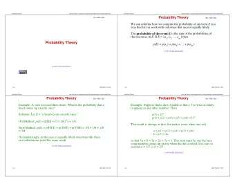
DATA MINING TECHNIQUES Review of Probability Theory Yijun Zhao Northeastern University spring 2015 Yijun Zhao DATA MINING TECHNIQUES Review of Probability Theory

Review of Probability Theory Based on ”Review of Probability Theory” from CS 229 Machine Learning, Stanford University (Handout posted on the course website) Yijun Zhao DATA MINING TECHNIQUES Review of Probability Theory

Elements of Probability Sample space Ω: the set of all the outcomes of an experiment Event space F : a collection of possible outcomes of an experiment. F ⊆ Ω. Probability measure: a function P : F → R that satisfies the following properties: P ( A ) ≥ 0 ∀ A ∈ F P (Ω) = 1 If A 1 , A 2 , . . . are disjoint events, then P ( ∪ i A i ) = � P ( A i ) i Yijun Zhao DATA MINING TECHNIQUES Review of Probability Theory

Properties of Probability If A ⊆ B = ⇒ P ( A ) ≤ P ( B ) P ( A ∩ B ) ≤ min ( P ( A ) , P ( B )) P ( A ∪ B ) ≤ P ( A ) + P ( B ) (Union Bound) P (Ω \ A ) = 1 − P ( A ) If A 1 , . . . , A k is a disjoint partition of Ω, then k � P ( A k ) = 1 i =1 Yijun Zhao DATA MINING TECHNIQUES Review of Probability Theory

Conditional Probability A conditional probability P ( A | B ) measures the probability of an event A after observing the occurrence of event B P ( A | B ) = P ( A ∩ B ) P ( B ) Two events A and B are independent iff P ( A | B ) = P ( A ) or equivalently, P ( A ∩ B ) = P ( A ) P ( B ) Yijun Zhao DATA MINING TECHNIQUES Review of Probability Theory

Conditional Probability Examples A math teacher gave her class two tests. 25% of the class passed both tests and 42% of the class passed the first test. What percent of those who passed the first test also passed the second test? In New England, 84% of the houses have a garage and 65% of the houses have a garage and a back yard. What is the probability that a house has a backyard given that it has a garage? Yijun Zhao DATA MINING TECHNIQUES Review of Probability Theory

Independent Events Examples What’s the probability of getting a sequence of 1,2,3,4,5,6 if we roll a dice six times? A school survey found that 9 out of 10 students like pizza. If three students are chosen at random with replacement, what is the probability that all three students like pizza? Yijun Zhao DATA MINING TECHNIQUES Review of Probability Theory

Random Variable A random variable X is a function that maps a sample space Ω to real values. Formally, X : Ω − → R Examples: Rolling one dice X = number on the dice at each roll Rolling two dice at the same time X = sum of the two numbers Yijun Zhao DATA MINING TECHNIQUES Review of Probability Theory

Random Variable A random variable can be continuous. E.g., X = the length of a randomly selected phone call (What’s the Ω?) X = amount of coke left in a can marked 12oz (What’s the Ω?) Yijun Zhao DATA MINING TECHNIQUES Review of Probability Theory

Probability Mass Function If X is a discrete random variable, we can specify a probability for each of its possible values using the probability mass function ( PMF ). Formally, a PMF is a function p : Ω − → R such that p ( x ) = P ( X = x ) Rolling a dice: p ( X = i ) = 1 i = 1 , 2 , . . . , 6 6 Rolling two dice at the same time: X = sum of the two numbers p ( X = 2) = 1 36 Yijun Zhao DATA MINING TECHNIQUES Review of Probability Theory

Probability Mass Function X ∼ Bernoulli ( p ), p ∈ [0 , 1] � if x = 1 p p ( x ) = 1 − p if x = 0 X ∼ Binomial ( n , p ), p ∈ [0 , 1] and n ∈ Z + � n � p x (1 − p ) n − x p ( x ) = x X ∼ Geometric ( p ), p > 0 p ( x ) = p (1 − p ) x − 1 X ∼ Poisson ( λ ), λ > 0 p ( x ) = e − λλ x x ! Yijun Zhao DATA MINING TECHNIQUES Review of Probability Theory

Probability Density Function If X is a continuous random variable, we can NOT specify a probability for each of its possible values (why?) We use a probability density function PDF to describe the relative likelihood for a random variable to take on a given value A ( PDF ) specifies the probability of X takes a value within a range. Formally, a PDF is a function f ( x ): Ω − → R such that � b P ( a < X < b ) = f ( x ) dx a Yijun Zhao DATA MINING TECHNIQUES Review of Probability Theory

Probability Density Function X ∼ uniform on [ a , b ]: 1 f ( x ) = b − a X ∼ N ( µ, σ ) : 2 π e − 1 2 σ 2 ( x − µ ) 2 1 f ( x ) = √ σ Yijun Zhao DATA MINING TECHNIQUES Review of Probability Theory

Joint Probability Mass Function If we have two discrete random variables X , Y , we can define their joint probability mass function ( PMF ) p XY : R 2 − → [0 , 1] as: p ( x , y ) = P ( X = x , Y = y ) where p ( x , y ) ≤ 1 and � � p ( x , y ) = 1 x ∈ X y ∈ Y X , Y : rolling two dice p ( x , y ) = 1 x , y = 1 , 2 , . . . , 6 36 X : rolling one dice Y : drawing a colored ball p (6 , green ) =? p (5 , red ) =? Yijun Zhao DATA MINING TECHNIQUES Review of Probability Theory

Joint Probability Density Function If we have two continuous random variables X , Y , we can define their joint probability density function ( PDF ) f XY : R 2 − → [0 , 1] as: � d � b P ( a < X < b , c < Y < d ) = f ( x , y ) dxdy c a 2D Gaussian Yijun Zhao DATA MINING TECHNIQUES Review of Probability Theory

Marginal Probability Mass Function How does the joint PMF over two discrete variables relate to the PMF for each variable separately? It turns out that � p ( x ) = p ( x , y ) y ∈ Y X , Y : rolling two dice p ( x , y ) = 1 x , y = 1 , 2 , . . . , 6 36 6 p ( x , y ) = 1 � p ( x ) = 6 y =1 Yijun Zhao DATA MINING TECHNIQUES Review of Probability Theory

Marginal Probability Density Function Similarly, we can obtain a marginal PDF (also called marginal density) for a continuous random variable from a joint PDF : � ∞ f ( x ) = f ( x , y ) dy −∞ Integrating out one variable in the 2D Gaussian gives a 1D Gaussian in either dimension Yijun Zhao DATA MINING TECHNIQUES Review of Probability Theory

Conditional Probability Distribution A conditional probability distribution defines the probability distribution over Y when we know that X must take on a certain value x Discrete case: conditional PMF p ( y | x ) = p ( x , y ) p ( x ) ⇐ ⇒ p ( x , y ) = p ( y | x ) p ( x ) Continuous case: conditional PDF f ( y | x ) = f ( x , y ) f ( x ) ⇐ ⇒ f ( x , y ) = f ( y | x ) f ( x ) Yijun Zhao DATA MINING TECHNIQUES Review of Probability Theory

Marginal vs. Conditional  Marginal probability:  Conditional probability: probability of rolling a 2 Yijun Zhao DATA MINING TECHNIQUES Review of Probability Theory

Bayes Rule We can express the joint probability in two ways: p ( x , y ) = p ( y | x ) p ( x ) p ( x , y ) = p ( x | y ) p ( y ) Bayes rule: p ( y | x ) = p ( x | y ) p ( y ) (discrete) p ( x ) f ( y | x ) = f ( x | y ) f ( y ) (continuous) f ( x ) Yijun Zhao DATA MINING TECHNIQUES Review of Probability Theory

Bayes Rule Application A patient underwent a HIV test and got a positive result. Suppose we know that Overall risk of having HIV in the population is 0.1% The test can accurately identify 98% of HIV infected patients The test can accurately identify 99% of healthy patients What’s the probability the person indeed infected HIV? Yijun Zhao DATA MINING TECHNIQUES Review of Probability Theory

Bayes Rule - Application We have two random variables here: X ∈ { + , −} : the outcome of the HIV test C ∈ { Y , N } : the patient has HIV or not We want to know: P ( C =Y | X =+ ) ? Apply Bayes rule: P ( C =Y | X =+) = P ( X =+ | C =Y) P ( C =Y) P ( X =+) P ( X =+ | C =Y) = 0 . 98 P ( C =Y) = 0 . 001 P ( X =+) = 0 . 98 ∗ 0 . 001+(1-0 . 99) ∗ 0 . 999 = 0 . 01097 Answer: 0 . 98 ∗ 0 . 001 / 0 . 01097 = 8 . 9% Yijun Zhao DATA MINING TECHNIQUES Review of Probability Theory

Bayes Rule Terminology P ( Y | X ) = P ( X | Y ) P ( Y ) P ( X ) P ( Y ): prior probability or, simply, prior P ( X | Y ): conditional probability or, likelihood P ( X ): marginal probability P ( Y | X ): posterior probability or, simply, posterior Yijun Zhao DATA MINING TECHNIQUES Review of Probability Theory

Independence Two random variables X and Y are independent iff For discrete random variables p ( x , y ) = p ( x ) p ( y ) ∀ x ∈ X , y ∈ Y For discrete random variables p ( y | x ) = p ( y ) ∀ y ∈ Y and p ( x ) � = 0 For continuous random variables f ( x , y ) = f ( x ) f ( y ) ∀ x , y ∈ R For continuous random variables f ( y | x ) = f ( y ) ∀ y ∈ R and f ( x ) � = 0 Yijun Zhao DATA MINING TECHNIQUES Review of Probability Theory

Multiple Random Variables Extend to multiple random variables : Joint Distribution (discrete): p ( x 1 , . . . , x n ) = P ( X 1 = x 1 , . . . , X n = x n ) Conditional Distribution (chain rule - discrete) p ( x 1 , . . . , x n ) = p ( x n | x 1 , . . . , x n − 1 ) p ( x 1 , . . . , x n − 1 ) = p ( x n | x 1 , . . . , x n − 1 ) p ( x n − 1 | x 1 , . . . , x n − 2 ) p ( x 1 , . . . , x n − 2 ) n � = p ( x 1 ) p ( x i | x 1 , . . . , x i − 1 ) i =2 (continuous case can be defined similarly using PDF ) Yijun Zhao DATA MINING TECHNIQUES Review of Probability Theory

Multiple Random Variables Independence: Discrete case: X 1 , . . . , X n are independent iff n p ( x 1 , . . . , x n ) = � p ( x i ) i =1 Continuous case: X 1 , . . . , X n are independent iff n f ( x 1 , . . . , x n ) = � f ( x i ) i =1 Yijun Zhao DATA MINING TECHNIQUES Review of Probability Theory