Continuous Distributions 1.8-1.9: Continuous Random Variables - PowerPoint PPT Presentation
Continuous Distributions 1.8-1.9: Continuous Random Variables 1.10.1: Uniform Distribution (Continuous) 1.10.4-5 Exponential and Gamma Distributions: Distance between crossovers Prof. Tesler Math 283 Fall 2019 Prof. Tesler Continuous
Continuous Distributions 1.8-1.9: Continuous Random Variables 1.10.1: Uniform Distribution (Continuous) 1.10.4-5 Exponential and Gamma Distributions: Distance between crossovers Prof. Tesler Math 283 Fall 2019 Prof. Tesler Continuous Distributions Math 283 / Fall 2019 1 / 33
Cumulative Distribution Function (CDF) Prof. Tesler Continuous Distributions Math 283 / Fall 2019 2 / 33
Cumulative Distribution Function (CDF) Discrete random variables The Cumulative Distribution Function (CDF) of PDF random variable X is P X ( k ) k F X ( x ) = P ( X � x ) 0 . 5 0 . 1 1 . 0 0 . 2 F X ( 1 . 5 ) = P ( X � 1 . 5 ) = P X ( 0 . 5 ) + P X ( 1 . 0 ) + P X ( 1 . 5 ) 1 . 5 0 . 3 = 0 . 1 + 0 . 2 + 0 . 3 = 0 . 6 2 . 0 0 . 1 2 . 5 0 . 1 3 . 0 0 . 2 In-between points with nonzero probability: F X ( 1 . 7 ) = P ( X � 1 . 7 ) = P ( X � 1 . 5 ) = F X ( 1 . 5 ) = 0 . 6 whereas the PDF there is 0 : P X ( 1 . 7 ) = 0 Similarly, F X ( k ) = F X ( 1 . 5 ) = 0 . 6 for 1 . 5 � k < 2 . 0 . Prof. Tesler Continuous Distributions Math 283 / Fall 2019 3 / 33
CDF outside of the range PDF P X ( k ) k 0 . 5 0 . 1 1 . 0 0 . 2 1 . 5 0 . 3 2 . 0 0 . 1 2 . 5 0 . 1 3 . 0 0 . 2 F X (− 1 ) = P ( X � − 1 ) = 0 (no points w/nonzero PDF) F X ( 5 ) = P ( X � 5 ) = 1 (has all of the points w/nonzero PDF) General case k → − ∞ F X ( k ) = 0 lim k → + ∞ F X ( k ) = 1 lim Prof. Tesler Continuous Distributions Math 283 / Fall 2019 4 / 33
CDF table PDF CDF P X ( k ) F X ( k ) k k k < 0 . 5 0 0 . 5 0 . 1 0 . 5 � k < 1 . 0 0 . 1 1 . 0 0 . 2 1 . 0 � k < 1 . 5 0 . 3 1 . 5 0 . 3 1 . 5 � k < 2 . 0 0 . 6 2 . 0 0 . 1 2 . 0 � k < 2 . 5 0 . 7 2 . 5 0 . 1 2 . 5 � k < 3 . 0 0 . 8 3 . 0 0 . 2 3 . 0 � k 1 Prof. Tesler Continuous Distributions Math 283 / Fall 2019 5 / 33
Using CDF table with various inequalities: � , > , < , � PDF CDF P X ( k ) F X ( k ) k k k < 0 . 5 0 0 . 5 0 . 1 0 . 5 � k < 1 . 0 0 . 1 1 . 0 0 . 2 1 . 0 � k < 1 . 5 0 . 3 1 . 5 0 . 3 1 . 5 � k < 2 . 0 0 . 6 2 . 0 0 . 1 2 . 0 � k < 2 . 5 0 . 7 2 . 5 0 . 1 2 . 5 � k < 3 . 0 0 . 8 3 . 0 0 . 2 3 . 0 � k 1 P ( X � 1 ) = 0 . 3 P ( X > 1 ) = 1 − P ( X � 1 ) = 0 . 7 P ( X < 1 ) = P ( X � 1 − ) = F X ( 1 − ) = 0 . 1 using infinitesimal notation from Calculus: 1 − is just below 1 , like 0 . 99999999 , but even closer. P ( X � 1 ) = 1 − P ( X < 1 ) = 1 − F X ( 1 − ) = 0 . 9 Prof. Tesler Continuous Distributions Math 283 / Fall 2019 6 / 33
Using CDF table on an interval PDF CDF P X ( k ) F X ( k ) k k k < 0 . 5 0 0 . 5 0 . 1 0 . 5 � k < 1 . 0 0 . 1 1 . 0 0 . 2 1 . 0 � k < 1 . 5 0 . 3 1 . 5 0 . 3 1 . 5 � k < 2 . 0 0 . 6 2 . 0 0 . 1 2 . 0 � k < 2 . 5 0 . 7 2 . 5 0 . 1 2 . 5 � k < 3 . 0 0 . 8 3 . 0 0 . 2 3 . 0 � k 1 F X ( 2 ) = P ( X � 2 ) = P X ( 0 . 5 ) + P X ( 1 . 0 ) + P X ( 1 . 5 ) + P X ( 2 . 0 ) F X ( 1 ) = P ( X � 1 ) = P X ( 0 . 5 ) + P X ( 1 . 0 ) P ( 1 < X � 2 ) = P X ( 1 . 5 ) + P X ( 2 . 0 ) = P ( X � 2 ) − P ( X � 1 ) = F X ( 2 ) − F X ( 1 ) = 0 . 7 − 0 . 3 = 0 . 4 Prof. Tesler Continuous Distributions Math 283 / Fall 2019 7 / 33
Converting intervals to the form P ( a < X � b ) PDF CDF P X ( k ) F X ( k ) k k k < 0 . 5 0 0 . 5 0 . 1 0 . 5 � k < 1 . 0 0 . 1 1 . 0 0 . 2 1 . 0 � k < 1 . 5 0 . 3 1 . 5 0 . 3 1 . 5 � k < 2 . 0 0 . 6 2 . 0 0 . 1 2 . 0 � k < 2 . 5 0 . 7 2 . 5 0 . 1 2 . 5 � k < 3 . 0 0 . 8 3 . 0 0 . 2 3 . 0 � k 1 The formula P ( a < X � b ) = F X ( b ) − F X ( a ) uses a < X (not a � X ) and X � b (not X < b ). Other formats must be converted to this: P ( 1 < X � 2 ) = F X ( 2 ) − F X ( 1 ) = 0 . 7 − 0 . 3 = 0 . 4 P ( 1 � X � 2 ) = P ( 1 − < X � 2 ) = F X ( 2 ) − F X ( 1 − ) = 0 . 7 − 0 . 1 = 0 . 6 P ( 1 < X < 2 ) = P ( 1 < X � 2 − ) = F X ( 2 − ) − F X ( 1 ) = 0 . 6 − 0 . 3 = 0 . 3 P ( 1 � X < 2 ) = P ( 1 − < X � 2 − ) = F X ( 2 − ) − F X ( 1 − ) = 0 . 6 − 0 . 1 = 0 . 5 Prof. Tesler Continuous Distributions Math 283 / Fall 2019 8 / 33
Continuous distributions Prof. Tesler Continuous Distributions Math 283 / Fall 2019 9 / 33
Continuous distributions Example Pick a real number x between 20 and 30 with all real values in [ 20 , 30 ] equally likely. Sample space: S = [ 20 , 30 ] Number of outcomes: | S | = ∞ Probability of each outcome: P ( X = x ) = 1 ∞ = 0 Yet, P ( X � 21 . 5 ) = 15 % Prof. Tesler Continuous Distributions Math 283 / Fall 2019 10 / 33
Continuous distributions The sample space S is often a subset of R n . We’ll do the 1-dimensional case S ⊂ R . The probability density function (PDF) f X ( x ) is defined differently than the discrete case: f X ( x ) is a real-valued function on S with f X ( x ) � 0 for all x ∈ S . � (vs. � f X ( x ) dx = 1 P X ( x ) = 1 for discrete) x ∈ S S � (vs. � The probability of event A ⊂ S is P ( A ) = f X ( x ) dx P X ( x ) ). x ∈ A A In n dimensions, use n -dimensional integrals instead. Notation: Uppercase F for CDF vs. lowercase f for pdf. Uniform distribution Let a < b be real numbers. The Uniform Distribution on [ a , b ] is that all numbers in [ a , b ] are “equally likely.” � 1 if a � x � b ; b − a More precisely, f X ( x ) = otherwise. 0 Prof. Tesler Continuous Distributions Math 283 / Fall 2019 11 / 33
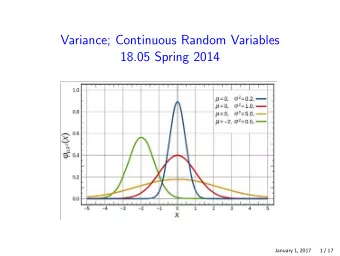
Uniform distribution (real case) The uniform distribution on [ 20 , 30 ] We could regard the sample space as [ 20 , 30 ] , or as all reals. 0.10 f X ( x ) � for 20 � x � 30 ; 1 / 10 f X ( x ) = 0.00 otherwise. 0 0 10 20 30 40 x � 20 � 21 . 5 21 . 5 10 dx = 0 + x 1 � P ( X � 21 . 5 ) = 0 dx + � 10 � 20 − ∞ 20 = 21 . 5 − 20 0.10 10 f X ( x ) = . 15 = 15 % 0.00 0 10 20 30 40 x Prof. Tesler Continuous Distributions Math 283 / Fall 2019 12 / 33
Cumulative distribution function (CDF) The Cumulative Distribution Function (CDF) of a random variable X is F X ( x ) = P ( X � x ) For a continuous random variable, � x ′ ( x ) F X ( x ) = P ( X � x ) = − ∞ f X ( t ) dt and f X ( x ) = F X The integral cannot have “ x ” as the name of the variable in both of F X ( x ) and f X ( x ) because one is the upper limit of the integral and the other is the integration variable. So we use two variables x , t . We can either write � x F X ( x ) = P ( X � x ) = f X ( t ) dt − ∞ or � t F X ( t ) = P ( X � t ) = f X ( x ) dx − ∞ Prof. Tesler Continuous Distributions Math 283 / Fall 2019 13 / 33
CDF of uniform distribution Uniform distribution on [ 20 , 30 ] � x For x < 20 : F X ( x ) = − ∞ 0 dt = 0 � 20 � x 10 dt = x − 20 1 For 20 � x < 30 : F X ( x ) = − ∞ 0 dt + 20 10 � 20 � 30 � x 1 For 30 � x : F X ( x ) = − ∞ 0 dt + 10 dt + 30 0 dt = 1 20 Together: if x < 20 if x < 20 0 0 x − 20 1 ′ ( x )= F X ( x )= f X ( x )= F X if 20 � x � 30 if 20 � x � 30 10 10 if x � 30 if x � 30 1 0 Prof. Tesler Continuous Distributions Math 283 / Fall 2019 14 / 33
PDF vs. CDF Probability density function Cumulative distribution function 1 0.10 F X ( x ) 0.5 f X ( x ) 0 0.00 0 10 20 30 40 0 10 20 30 40 x x � F X ( x ) = . 1 if 20 � x � 30 ; f X ( x )= if x < 20 ; 0 otherwise. 0 It’s discontinuous at x = 20 ( x − 20 ) / 10 if 20 � x � 30 ; and 30 . if x � 30 . 1 PDF is derivative of CDF: CDF is integral of PDF: � x ′ ( x ) f X ( x ) = F X F X ( x ) = f X ( t ) dt − ∞ Prof. Tesler Continuous Distributions Math 283 / Fall 2019 15 / 33
PDF vs. CDF: Second example Probability density function Cumulative distribution function 1 density f R (r) 0.6 F R (r) 0.4 0.5 0.2 0 0 0 1 2 3 0 1 2 3 r r � 2 r / 9 if 0 � r < 3 ; if r < 0 ; 0 f R ( r )= r 2 / 9 if r � 0 or r > 3 0 F R ( r ) = if 0 � r � 3 ; It’s discontinuous at r = 3 . if r � 3 . 1 PDF is derivative of CDF: CDF is integral of PDF: � r ′ ( r ) f R ( r ) = F R F R ( r ) = f R ( t ) dt − ∞ Prof. Tesler Continuous Distributions Math 283 / Fall 2019 16 / 33
Probability of an interval Compute P (− 1 � R � 2 ) from the PDF and also from the CDF Computation from the PDF � 2 � 0 � 2 P (− 1 � R � 2 ) = f R ( r ) dr = f R ( r ) dr + f R ( r ) dr − 1 − 1 0 � 0 � 2 2 r = 0 dr + 9 dr − 1 0 = 2 2 − 0 2 � 2 � r 2 � = 4 � = 0 + � 9 9 9 � r = 0 Computation from the CDF P (− 1 � R � 2 ) = P (− 1 − < R � 2 ) = F R ( 2 ) − F R (− 1 − ) = 2 2 9 − 0 = 4 9 Prof. Tesler Continuous Distributions Math 283 / Fall 2019 17 / 33
Continuous vs. discrete random variables Cumulative distribution function Cumulative distribution function 1 1 F X (x) F R (r) 0.5 0.5 0 0 0 1 2 3 ! 1 0 1 2 r x In a continuous distribution: The probability of an individual point is 0 : P ( R = r ) = 0 . So, P ( R � r ) = P ( R < r ) , i.e., F R ( r ) = F R ( r − ) . The CDF is continuous. (In a discrete distribution, the CDF is discontinuous due to jumps at the points with nonzero probability.) P ( a < R < b )= P ( a � R < b ) = P ( a < R � b ) = P ( a � R � b ) = F R ( b ) − F R ( a ) Prof. Tesler Continuous Distributions Math 283 / Fall 2019 18 / 33
Recommend
More recommend
Explore More Topics
Stay informed with curated content and fresh updates.
