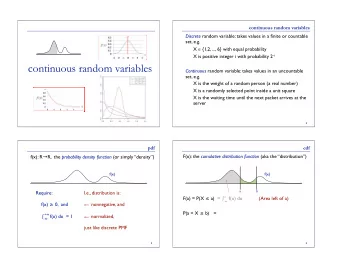
Continuous Random Variables Recall: A continuous random variable X - PowerPoint PPT Presentation

ST 380 Probability and Statistics for the Physical Sciences Continuous Random Variables Recall: A continuous random variable X satisfies: its range is the union of one or more real number intervals; 1 P ( X = c ) = 0 for every c in the range of X . 2 Examples: The depth of a lake at a randomly chosen location. The pH of a random sample of effluent. The precipitation on a randomly chosen day is not a continuous random variable: its range is [0 , ∞ ), and P ( X = c ) = 0 for any c > 0, but P ( X = 0) > 0. 1 / 12 Continuous Random Variables Probability Density Function

ST 380 Probability and Statistics for the Physical Sciences Discretized Data Suppose that we measure the depth of the lake, but round the depth off to some unit. The rounded value Y is a discrete random variable; we can display its probability mass function as a bar graph, because each mass actually represents an interval of values of X . In R source("discretize.R") discretize(0.5) 2 / 12 Continuous Random Variables Probability Density Function

ST 380 Probability and Statistics for the Physical Sciences As the rounding unit becomes smaller, the bar graph more accurately represents the continuous distribution: discretize(0.25) discretize(0.1) When the rounding unit is very small, the bar graph approximates a smooth function: discretize(0.01) plot(f, from = 1, to = 5) 3 / 12 Continuous Random Variables Probability Density Function

ST 380 Probability and Statistics for the Physical Sciences The probability that X is between two values a and b , P ( a ≤ X ≤ b ), can be approximated by P ( a ≤ Y ≤ b ). Because Y is discrete, P ( a ≤ Y ≤ b ) is the sum of the areas of the corresponding bars in the graph. As the rounding unit becomes smaller, the sum of the areas of the bars approaches the integral of the smooth function. In the limit, � b P ( a ≤ X ≤ b ) = f ( x ) d x . a 4 / 12 Continuous Random Variables Probability Density Function

ST 380 Probability and Statistics for the Physical Sciences The smooth function f ( x ) is called a probability density function (pdf). Clearly f ( x ) must satisfy: f ( x ) ≥ 0 , −∞ < x < ∞ ; (1) � ∞ f ( x ) d x = 1 . (2) −∞ Any f ( x ) satisfying these two conditions could be the pdf of some continuous random variable. 5 / 12 Continuous Random Variables Probability Density Function

ST 380 Probability and Statistics for the Physical Sciences Uniform Distribution A bee leaves its hive to forage for blossom that will provide nectar. If the bee has no prior information, it searches in a random direction. If X is the direction, measured from North clockwise in degrees, then X is equally likely to be any value in [0 , 360). More precisely, if 0 ≤ a < b < 360, then � b 1 P ( a ≤ X ≤ b ) = b − a 360 = 360 d x . a So the pdf is f ( x ) = 1 / 360 , 0 ≤ x < 360, and zero otherwise. 6 / 12 Continuous Random Variables Probability Density Function

ST 380 Probability and Statistics for the Physical Sciences Cumulative Distribution Function The cumulative distribution function F ( x ) of any random variable X is defined as F ( x ) = P ( X ≤ x ) , −∞ < x < ∞ . Earlier, for a continuous random variable X , � b P ( a ≤ X ≤ b ) = f ( y ) d y , a so � x F ( x ) = P ( X ≤ x ) = f ( y ) d y . −∞ 7 / 12 Continuous Random Variables Cumulative Distribution Function

ST 380 Probability and Statistics for the Physical Sciences Conversely, f ( x ) = dF ( x ) = F ′ ( x ) . dx For the uniform distribution on [0 , 1), � 1 0 ≤ x < 1 f ( x ) = 0 otherwise and  0 x < 0 � x   F ( x ) = f ( y ) d y = 0 ≤ x < 1 x −∞  1 x ≥ 1  8 / 12 Continuous Random Variables Cumulative Distribution Function

ST 380 Probability and Statistics for the Physical Sciences Percentiles The (100 p ) th percentile of X is the value that X falls below with probability p . That is, it is the value η ( p ) that satisfies P [ X ≤ η ( p )] = p . In terms of the cdf, � η ( p ) p = F [ η ( p )] = f ( y ) d y . −∞ 9 / 12 Continuous Random Variables Cumulative Distribution Function

ST 380 Probability and Statistics for the Physical Sciences Median and Quartiles Most commonly used percentiles: The median is the 50 th percentile, P ( X ≤ median) = 1 2 . The upper and lower quartiles are the 75 th and 25 th percentiles, respectively, P ( X ≤ upper quartile) = 3 4 , P ( X ≤ lower quartile) = 1 4 . 10 / 12 Continuous Random Variables Cumulative Distribution Function

ST 380 Probability and Statistics for the Physical Sciences Expected Value Recall that the expected value of a discrete random variable is the average of its values, weighted by their probabilities. For a continuous random variable, expected value is defined the same way, but the average must be computed as an integral instead of a sum : � ∞ µ X = E ( X ) = x · f ( x ) d x . −∞ More generally, for a function h ( X ), � ∞ µ h ( X ) = E [ h ( X )] = h ( x ) · f ( x ) d x . −∞ 11 / 12 Continuous Random Variables Expected Value

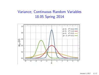
ST 380 Probability and Statistics for the Physical Sciences Variance and Standard Deviation As for a discrete random variable, the variance of X is σ 2 ( X − µ X ) 2 � � X = V ( X ) = E and the standard deviation is � σ X = V ( X ) . But the expected value is now given by an integral: � ∞ ( x − µ X ) 2 · f ( x ) d x � ( X − µ X ) 2 � E = −∞ 12 / 12 Continuous Random Variables Expected Value