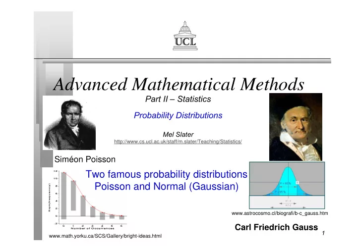

Advanced Mathematical Methods Part II – Statistics Probability Distributions Mel Slater http://www.cs.ucl.ac.uk/staff/m.slater/Teaching/Statistics/ Siméon Poisson Two famous probability distributions Poisson and Normal (Gaussian) www.astrocosmo.cl/biografi/b-c_gauss.htm Carl Friedrich Gauss 1 www.math.yorku.ca/SCS/Gallery/bright-ideas.html
Outline � Random variables � Probability Distributions � Summary Measures � Moment Generating Functions � (Common Distributions) � In today’s lecture we learn some definitions that are critical for the rest of the course. 2
Random Variables � Events are subsets of the domain of elementary events � Very often the ‘event’ is expressed in numerical form • The number of people out of n who experience high presence in a VE is x • The number of heads on n tosses of a coin is x • The heart rate of a person when subject to a certain stimulii will increase by x 3
Random Variables � A random variable is a variable that has a probability associated with each possible value it can take (discrete case) � Or which has a probability associated with any subset of the range of values it can take. 4
Random Variable Examples � For example: X is the number of heads in two tosses of a coin, then • p(X=0) = ¼ {TT} • p(X=1) = ½ {HT,TH} • p(X=2) = ¼ {HH} � Y is the number of cars that pass a spot on a road during 1 hour. The range of values of X = 0,1,2,3,… � Z is the time between two successive cars passing a spot on a road, then Y ≥ 0 (a continuous r.v.). 5
Distribution Function � For any r.v. X, define: • F(x) = p(X ≤ x) • The probability that X will have a value of no more than x. � Suppose the range of X is [a,b]. Then it follows from the axioms of probability that: • F(a) = 0 • F(b) = 1 • F(x+h) – F(x) ≥ 0 for any h ≥ 0. 6
Discrete Distributions � When X is a discrete r.v. with integer values then, define • f(x) = F(x+1) – F(x) � Note f(x) = p(X=x) • the probability that X takes the value x exactly. � f is called the probability density function (pdf). 7
Continuous Distributions � Suppose X is a continuous r.v., and consider � f(x) is also the p.d.f. and may be interpreted as f(x)dx being the probability that X takes a value in a small interval around x. 8
Distributions and Probability � Note that 9
Properties of pdf’s where D is the range of X. Any function that satisfies these properties may serve as a pdf. 10
Summary Measures � Expectation (Mean) � In general if g is any function of X then � It is easy to show from the definition that • E(a + bg(X)) = a + bE(g(X)) for constants a,b. 11
Variance � The variance is a measure of variation about the mean:- � If we write Then it can be shown that 12
Moments about Origin & Mean � rth moment about the origin is defined as � rth moment about the mean as: 13
Mean and Variance as Moments � Show:- � Note that some distributions will have no finite moments. � The moments of a distribution (if they exist) completely characterise the distribution. 14
Moment Generating Functions � Different way to specify a distribution � Expand the exponential to get: � So the moments are coefficients of powers of t over the factorials! 15
MGF Properties (prove by differentiation) where g(X) is any function of X 16
Distributions � There are many ‘standard’ distributions � These occur again and again in scientific applications � And are given special names. � We will consider several now. 17
Discrete Uniform Distribution � X is a r.v. which has domain {1,2,…,n} � Each value of X is considered equally likely. � P(X=x) = 1/n, x = 1,2,…,n • (there are many possible versions of this distribution) � Ex: From the definition find E(X), Var(X) and M X (t) 18
Continuous Uniform Distribution � X is equally likely to take any value in the continuous range [a,b]: � The MGF can be found to be: � From this it is easy to find the mean E(X) and variance Var(X). 19
Binomial Distribution � There are two exclusive outcomes to an experimental trial labelled S or F. � P(S) = p, P(F) = 1-p = q. � Each trial is independent. � There are n trials. � X is the number of S outcomes. � X ∈ {0,1,2,…,n} 20
Binomial Distribution � Any particular outcome with x S’s has probability p x q n-x . � Combinatorial theory shows that there are n!/x!(n-x)! such outcomes with x S’s and n-x Fs. � Hence:- � With MGF � With E(X) = np and Var(X) = npq 21
Poisson Distribution � An event happens at random in time • E.g., failures of the tracking system in the ‘Cave’ • E.g., a customer enters a shop • E.g., a train arrives at a station � X is the number of events per unit time � X = 0,1,2,… 22
Exponential Distribution � Same setup as for Poisson but let Y be the time between successive events. � MGF is: � Expanding the MGF as a power series it is easy to see that: 23
Other Distributions… � Check out each of the following in the notes: • Beta distribution – Distribution proportions i.e. in [0,1] • Negative binomial distribution – The number of trials before x successes are achieved in the binomial setup • Gamma Distribution – This is the time between k successive events in the Poisson setup. � For each case look at the derivation, mean, variance and MGF 24
Standard Statistical Distributions � There are a number of distributions that regularly appear in statistical practice: • Normal (Gaussian) • Chi-squared χ 2 • t-distribution • F distribution � With MATLAB you should learn how to find probabilities from these distributions. 25
Normal Distribution � Occurs very often in nature and in social situations – arises from an ‘averaging’ process. � The mean E(X) = µ � Var(X) = σ 2 26
Standard Normal � X ~ N( µ , σ 2 ) � When µ = 0 and σ 2 = 1 this is called the Standard Normal distribution. � It is easy to show that when X ~ N( µ , σ 2 ) � Then Z = (X- µ )/ σ ~ N(0,1) � Then eg, • P(X > a) = P(Z > (a- µ )/ σ ) • and Z is tabulated (or available in MATLAB) � Typically we use P(Z<z) = F(z) the cummulative probability distribution (distribution function). 27
Chi-Squared χ 2 Distribution � Let X be a r.v. which is formed by the sum of squares of n independent N(0,1) variables. � X ~ χ 2 (n) distribution where n called the ‘degrees of freedom’. � Use MATLAB to learn how to look up probabilities for this distribution. 28
t-Distribution � Suppose Z ~ N(0,1) � X ~ χ 2 (n) � Suppose Z and X are independent. � Then t = Z/(X/n) ~ t-distribution with n degrees of freedom. � Learn how to use MATLAB to look up probabilities for this distribution. 29
F-Distribution � Suppose X1 ~ χ 2 (n1) � Suppose X2 ~ χ 2 (n2) • X1 and X2 are independent � Then • F = (X1/n1) / (X2/n2) ~ F(n1,n2) distribution • Where n1 and n2 are called the degrees of freedom of numerator and denominator. � Learn how to look up probabilities under this distribution using MATLAB. 30
Recommend
More recommend