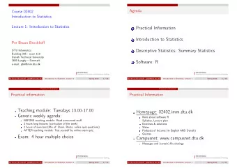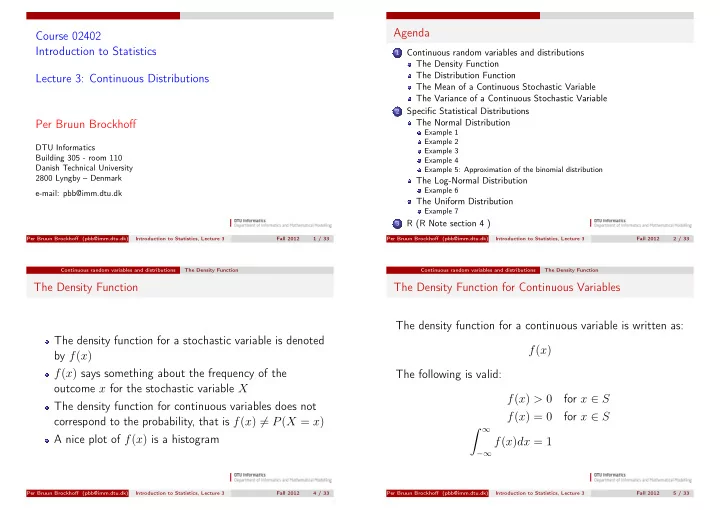
Agenda Course 02402 Introduction to Statistics Continuous random - PowerPoint PPT Presentation

Agenda Course 02402 Introduction to Statistics Continuous random variables and distributions 1 The Density Function The Distribution Function Lecture 3: Continuous Distributions The Mean of a Continuous Stochastic Variable The Variance of a Continuous Stochastic Variable Specific Statistical Distributions 2 The Normal Distribution Per Bruun Brockhoff Example 1 Example 2 DTU Informatics Example 3 Building 305 - room 110 Example 4 Danish Technical University Example 5: Approximation of the binomial distribution 2800 Lyngby – Denmark The Log-Normal Distribution Example 6 e-mail: pbb@imm.dtu.dk The Uniform Distribution Example 7 R (R Note section 4 ) 3 Per Bruun Brockhoff (pbb@imm.dtu.dk) Introduction to Statistics, Lecture 3 Fall 2012 1 / 33 Per Bruun Brockhoff (pbb@imm.dtu.dk) Introduction to Statistics, Lecture 3 Fall 2012 2 / 33 Continuous random variables and distributions The Density Function Continuous random variables and distributions The Density Function The Density Function The Density Function for Continuous Variables The density function for a continuous variable is written as: The density function for a stochastic variable is denoted f ( x ) by f ( x ) f ( x ) says something about the frequency of the The following is valid: outcome x for the stochastic variable X f ( x ) > 0 for x ∈ S The density function for continuous variables does not f ( x ) = 0 for x ∈ S correspond to the probability, that is f ( x ) � = P ( X = x ) � ∞ A nice plot of f ( x ) is a histogram f ( x ) dx = 1 −∞ Per Bruun Brockhoff (pbb@imm.dtu.dk) Introduction to Statistics, Lecture 3 Fall 2012 4 / 33 Per Bruun Brockhoff (pbb@imm.dtu.dk) Introduction to Statistics, Lecture 3 Fall 2012 5 / 33

Continuous random variables and distributions The Distribution Function Continuous random variables and distributions The Mean of a Continuous Stochastic Variable The Distribution Function The Mean of a Continuous Stochastic Variable The distribution function for a continuous stochastic variable is denoted by F ( x ) . The distribution function corresponds to the cumulative The mean of a continuous stochastic variable is calculated density function: as: � µ = x · f ( x ) dx F ( x ) = P ( X ≤ x ) S where S is the sample space of X � x F ( x ) = f ( t ) dt t = −∞ A nice plot of F ( x ) is the cumulative distribution plot Per Bruun Brockhoff (pbb@imm.dtu.dk) Introduction to Statistics, Lecture 3 Fall 2012 6 / 33 Per Bruun Brockhoff (pbb@imm.dtu.dk) Introduction to Statistics, Lecture 3 Fall 2012 7 / 33 Continuous random variables and distributions The Variance of a Continuous Stochastic Variable Specific Statistical Distributions The Variance of a Continuous Stochastic Variable Specific Statistical Distributions The variance of a continuous stochastic variable is A number of statistical distributions exist that can be calculated as: used to describe and analyze different kind of problems � Now we consider continuous distributions σ 2 = ( x − µ ) 2 · f ( x ) dx The normal distribution S The log-normal distribution The uniform distribution where S is the sample space of X Per Bruun Brockhoff (pbb@imm.dtu.dk) Introduction to Statistics, Lecture 3 Fall 2012 8 / 33 Per Bruun Brockhoff (pbb@imm.dtu.dk) Introduction to Statistics, Lecture 3 Fall 2012 10 / 33

Specific Statistical Distributions The Normal Distribution Specific Statistical Distributions The Normal Distribution The Normal Distribution The Normal Distribution The Normal Distribution 0.5 0.45 X ∼ N ( µ, σ 2 ) 0.4 Density function: 0.35 2 π e − ( x − µ )2 1 f ( x ) = 0.3 √ 2 σ 2 Density, f(x) σ Mean value: 0.25 0.2 µ = µ 0.15 Variance: σ 2 = σ 2 0.1 0.05 Table 3 for F ( x ) 0 −5 −4 −3 −2 −1 0 1 2 3 4 5 x Per Bruun Brockhoff (pbb@imm.dtu.dk) Introduction to Statistics, Lecture 3 Fall 2012 11 / 33 Per Bruun Brockhoff (pbb@imm.dtu.dk) Introduction to Statistics, Lecture 3 Fall 2012 12 / 33 Specific Statistical Distributions The Normal Distribution Specific Statistical Distributions The Normal Distribution The Normal Distribution The Normal Distribution The Normal Distribution N(0,1 2 ) Comparison of two normal distributions with different means and same variance 0.45 0.45 N(0,1 2 ) N(5,1 2 ) 0.4 0.4 0.35 0.35 0.3 0.3 Density, f(x) 0.25 0.25 0.2 0.2 0.15 0.15 0.1 0.1 0.05 0.05 0 0 −3 σ −2 σ − σ µ σ 2 σ 3 σ −0.05 −0.05 −5 −4 −3 −2 −1 0 1 2 3 4 5 −5 0 5 10 x Per Bruun Brockhoff (pbb@imm.dtu.dk) Introduction to Statistics, Lecture 3 Fall 2012 13 / 33 Per Bruun Brockhoff (pbb@imm.dtu.dk) Introduction to Statistics, Lecture 3 Fall 2012 14 / 33

Specific Statistical Distributions The Normal Distribution Specific Statistical Distributions The Normal Distribution The Normal Distribution The Normal Distribution Comparison of three normal distributions with same mean and different variance A normal distribution with mean value 0 and variance 1, 0.5 that is: 0.4 Z ∼ N (0 , 1 2 ) Density, f(x) 0.3 is called the standard normal distribution 0.2 An arbitrary normally distributed variable X ∼ N ( µ, σ 2 ) can be standardized by 0.1 0 Z = X − µ −10 −8 −6 −4 −2 0 2 4 6 8 10 σ x Per Bruun Brockhoff (pbb@imm.dtu.dk) Introduction to Statistics, Lecture 3 Fall 2012 15 / 33 Per Bruun Brockhoff (pbb@imm.dtu.dk) Introduction to Statistics, Lecture 3 Fall 2012 16 / 33 Specific Statistical Distributions The Normal Distribution Specific Statistical Distributions The Normal Distribution Example 1 Example 1 A weight has a measurement error, E , that can be b) What is the probability that the weight measures at least described by a standard normal disrtribution, i.e. 2 grams too much? E ∼ N (0 , 1 2 ) c) What is the probability that the weight measures at most ± 1 gram wrong? that is, mean µ = 0 and standard deviation σ = 1 gram. We now measure the weight of a single piece a) What is the probability that the weight measures at least 2 grams too little? Per Bruun Brockhoff (pbb@imm.dtu.dk) Introduction to Statistics, Lecture 3 Fall 2012 17 / 33 Per Bruun Brockhoff (pbb@imm.dtu.dk) Introduction to Statistics, Lecture 3 Fall 2012 18 / 33

Specific Statistical Distributions The Normal Distribution Specific Statistical Distributions The Normal Distribution Example 2 Example 3 It is assumed that among a group af elementary school It is assumed that among a group af elementary school teachers, the salary distribution can be described as a teachers, the salary distribution can be described as a normal distribution with mean µ = 280 . 000 and standard normal distribution with mean µ = 290 . 000 and standard deviation σ = 10 . 000 . deviation σ = 4 . 000 . a) What is the probability that a randomly selected teacher a) What is the probability that a randomly selected teacher earns more than 300.000? earns more than 300.000? Per Bruun Brockhoff (pbb@imm.dtu.dk) Introduction to Statistics, Lecture 3 Fall 2012 19 / 33 Per Bruun Brockhoff (pbb@imm.dtu.dk) Introduction to Statistics, Lecture 3 Fall 2012 20 / 33 Specific Statistical Distributions The Normal Distribution Specific Statistical Distributions The Normal Distribution Example 4 Example 5: Approximation of the binomial distribution It is assumed that among a group af elementary school In a dose-response experiment with 80 rats, it is assumed teachers, the salary distribution can be described as a that the probability that a rat survives the experiment is normal distribution with mean µ = 290 . 000 and standard p = 0 . 5 . deviation σ = 4 . 000 . a) What is the probability that at most 30 rats die in the a) Give the salary interval that covers 95% of all teachers’ experiment? salary b) What is the probability that between 38 and 42 rats die in the experiment? Per Bruun Brockhoff (pbb@imm.dtu.dk) Introduction to Statistics, Lecture 3 Fall 2012 21 / 33 Per Bruun Brockhoff (pbb@imm.dtu.dk) Introduction to Statistics, Lecture 3 Fall 2012 22 / 33

Specific Statistical Distributions The Log-Normal Distribution Specific Statistical Distributions The Log-Normal Distribution The Log-Normal Distribution The Log-Normal Distribution The Log−Normal Distribution LN(1,1) 0.25 X ∼ LN ( α, β ) 0.2 Density function: LN(1,1) 2 π x − 1 e − ( ln ( x ) − α ) 2 / 2 β 2 x > 0 , β > 0 � 1 √ 0.15 Density, f(x) f ( x ) = β 0 otherwise 0.1 Mean: µ = e α + β 2 / 2 0.05 Variance: σ 2 = e 2 α + β 2 ( e β 2 − 1) 0 0 5 10 15 20 25 30 x Per Bruun Brockhoff (pbb@imm.dtu.dk) Introduction to Statistics, Lecture 3 Fall 2012 23 / 33 Per Bruun Brockhoff (pbb@imm.dtu.dk) Introduction to Statistics, Lecture 3 Fall 2012 24 / 33 Specific Statistical Distributions The Log-Normal Distribution Specific Statistical Distributions The Log-Normal Distribution The Log-Normal Distribution Example 6 The particle size ( µm ) in a compoundi is assumed to follow a Log-normal distribution. We have the oberservations: A log-normally distributed variable Y ∼ LN ( α, β ) can be 2.2 3.4 1.6 0.8 2.7 3.3 1.6 2.8 1.9 transformed into a standard normally distributed variable X by: We take the logarithm of the data and achieve: X = ln ( Y ) − α 0.8 1.2 0.5 -0.2 1.0 1.2 0.5 1.0 0.6 β and then: from which we get: ¯ x = 0 . 733 and s = 0 . 44 . X ∼ N (0 , 1 2 ) What is the proportion of particles with a size in the interval [2; 3] Per Bruun Brockhoff (pbb@imm.dtu.dk) Introduction to Statistics, Lecture 3 Fall 2012 25 / 33 Per Bruun Brockhoff (pbb@imm.dtu.dk) Introduction to Statistics, Lecture 3 Fall 2012 26 / 33