Overview Course 02402 Introduction to Statistics Running example: - PowerPoint PPT Presentation

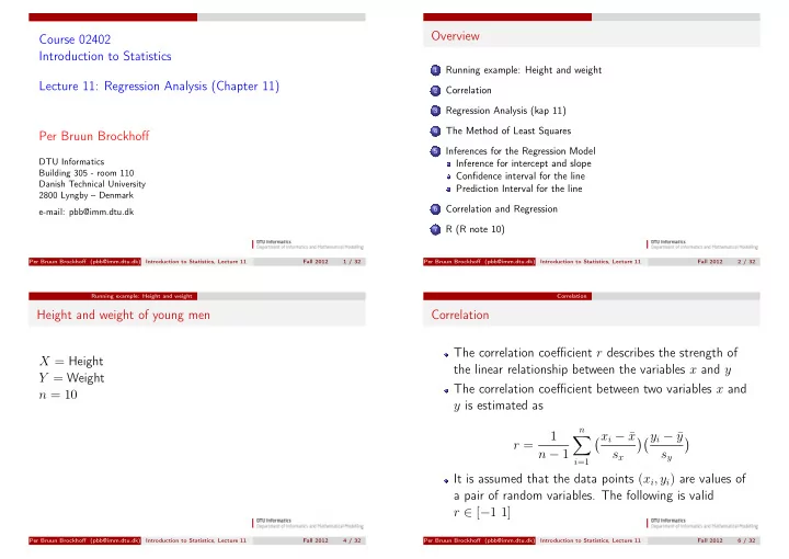
Overview Course 02402 Introduction to Statistics Running example: Height and weight 1 Lecture 11: Regression Analysis (Chapter 11) Correlation 2 Regression Analysis (kap 11) 3 The Method of Least Squares 4 Per Bruun Brockhoff Inferences for the Regression Model 5 DTU Informatics Inference for intercept and slope Building 305 - room 110 Confidence interval for the line Danish Technical University Prediction Interval for the line 2800 Lyngby – Denmark Correlation and Regression 6 e-mail: pbb@imm.dtu.dk R (R note 10) 7 Per Bruun Brockhoff (pbb@imm.dtu.dk) Introduction to Statistics, Lecture 11 Fall 2012 1 / 32 Per Bruun Brockhoff (pbb@imm.dtu.dk) Introduction to Statistics, Lecture 11 Fall 2012 2 / 32 Running example: Height and weight Correlation Height and weight of young men Correlation The correlation coefficient r describes the strength of X = Height the linear relationship between the variables x and y Y = Weight The correlation coefficient between two variables x and n = 10 y is estimated as n 1 � x i − ¯ x �� y i − ¯ y � � r = n − 1 s x s y i =1 It is assumed that the data points ( x i , y i ) are values of a pair of random variables. The following is valid r ∈ [ − 1 1] Per Bruun Brockhoff (pbb@imm.dtu.dk) Introduction to Statistics, Lecture 11 Fall 2012 4 / 32 Per Bruun Brockhoff (pbb@imm.dtu.dk) Introduction to Statistics, Lecture 11 Fall 2012 6 / 32

Correlation Regression Analysis (kap 11) Correlations computations Regression Analysis (Chapter 11) We assume that Y is a stochastic variable. We are interested in modelling Y ’s dependency on an explanatory variable x We look at a linear relationship between Y and x , that is a regression model on the form Y = α + βx + ε Per Bruun Brockhoff (pbb@imm.dtu.dk) Introduction to Statistics, Lecture 11 Fall 2012 7 / 32 Per Bruun Brockhoff (pbb@imm.dtu.dk) Introduction to Statistics, Lecture 11 Fall 2012 9 / 32 Regression Analysis (kap 11) Regression Analysis (kap 11) Simple Linear Regression Simple Linear Regression Y = α + βx + ε * ���� � �� � * residual model * * Y dependent variable x independent variable * * * α intercept with Y-axis * β slope * ε residual (random error) Per Bruun Brockhoff (pbb@imm.dtu.dk) Introduction to Statistics, Lecture 11 Fall 2012 10 / 32 Per Bruun Brockhoff (pbb@imm.dtu.dk) Introduction to Statistics, Lecture 11 Fall 2012 11 / 32

The Method of Least Squares The Method of Least Squares The Method of Least Squares The Method of Least Squares Scatterplot of x vs. Y 200 Assume we have the following observations 180 160 x 1 2 3 4 5 6 7 8 9 10 11 12 140 y 16 35 45 64 86 96 106 124 134 156 164 182 120 100 Is there a relationship between x and y ? Y 80 We propose a model on the form ˆ y = a + bx 60 How do we estimate a and b ? 40 20 0 0 2 4 6 8 10 12 x Per Bruun Brockhoff (pbb@imm.dtu.dk) Introduction to Statistics, Lecture 11 Fall 2012 13 / 32 Per Bruun Brockhoff (pbb@imm.dtu.dk) Introduction to Statistics, Lecture 11 Fall 2012 14 / 32 The Method of Least Squares The Method of Least Squares The Method of Least Squares The Method of Least Squares We define Regression Model 200 180 n 160 � x ) 2 S xx = ( x i − ¯ 140 i =1 120 n � Y 100 y ) 2 S yy = ( y i − ¯ 80 i =1 n 60 � S xy = ( x i − ¯ x )( y i − ¯ y ) 40 i =1 20 0 0 2 4 6 8 10 12 x Per Bruun Brockhoff (pbb@imm.dtu.dk) Introduction to Statistics, Lecture 11 Fall 2012 15 / 32 Per Bruun Brockhoff (pbb@imm.dtu.dk) Introduction to Statistics, Lecture 11 Fall 2012 16 / 32

The Method of Least Squares The Method of Least Squares The Method of Least Squares The Method of Least Squares In the example we get a and b are determined by b = S xy n � x ) 2 = 143 S xx = ( x i − ¯ S xx i =1 n a = ¯ y − b · ¯ x � y ) 2 = 31533 S yy = ( y i − ¯ a and b are the values that give the regression line that i =1 n minimizes the squared distance between the points and � S xy = ( x i − ¯ x )( y i − ¯ y ) = 2119 the line i =1 a is an estimate for α and b is an estimate for β along with ¯ x = 6 . 50 and ¯ y = 100 . 67 Per Bruun Brockhoff (pbb@imm.dtu.dk) Introduction to Statistics, Lecture 11 Fall 2012 17 / 32 Per Bruun Brockhoff (pbb@imm.dtu.dk) Introduction to Statistics, Lecture 11 Fall 2012 18 / 32 The Method of Least Squares Inferences for the Regression Model The Method of Least Squares Inferences for the Regression Model We assume that the observed data ( Y i , x i ) can be described by the model Estimates for α and β : b = S xy = 2119 Y i = α + βx i + ε i 143 = 14 . 82 S xx where it is assumed that ε i are independent normally distributed stochastic variables with mean 0 and constant a = ¯ y − b · ¯ x = 100 . 67 − 14 . 82 · 6 . 50 = 4 . 34 variance σ 2 The model is: An estimate of σ 2 is y = 4 . 34 + 14 . 82 · x ˆ e = S yy − ( S xy ) 2 /S xx s 2 n − 2 Per Bruun Brockhoff (pbb@imm.dtu.dk) Introduction to Statistics, Lecture 11 Fall 2012 19 / 32 Per Bruun Brockhoff (pbb@imm.dtu.dk) Introduction to Statistics, Lecture 11 Fall 2012 21 / 32

Inferences for the Regression Model Inference for intercept and slope Inferences for the Regression Model Inference for intercept and slope Inference for intercept and slope Inferences for intercept and slope We want to test the hypotheses about the intercept with We want to test a hypothesis about the slope β the y-axis H 0 : β = b H 0 : α = a H 1 : β � = b H 1 : α � = a The test statistic is The test statistic is t = ( b − β ) � � S xx t = ( a − α ) nS xx s e s e S xx + n (¯ x ) 2 The critical value is found in the t-distribution, t α/ 2 ( n − 2) The critical value is found in the t-distribution, t α/ 2 ( n − 2) Per Bruun Brockhoff (pbb@imm.dtu.dk) Introduction to Statistics, Lecture 11 Fall 2012 22 / 32 Per Bruun Brockhoff (pbb@imm.dtu.dk) Introduction to Statistics, Lecture 11 Fall 2012 23 / 32 Inferences for the Regression Model Inference for intercept and slope Inferences for the Regression Model Confidence interval for the line Confidence Intervals for α and β Confidence Interval for α + βx 0 Confidence interval for α � A confidence interval for α + βx 0 corresponds to a n + (¯ 1 x ) 2 confidence interval at the point x 0 a ± t α/ 2 · s e S xx � n + ( x 0 − ¯ 1 x ) 2 Confidence interval for β ( a + bx 0 ) ± t α/ 2 · s e S xx 1 b ± t α/ 2 · s e √ S xx Per Bruun Brockhoff (pbb@imm.dtu.dk) Introduction to Statistics, Lecture 11 Fall 2012 24 / 32 Per Bruun Brockhoff (pbb@imm.dtu.dk) Introduction to Statistics, Lecture 11 Fall 2012 25 / 32

Inferences for the Regression Model Prediction Interval for the line Correlation and Regression Prediction Interval for α + βx 0 Correlation and Regression Correlation coefficient and slope: √ S xx r 2 = S xx A prediction interval for α + βx 0 corresponds to a b 2 r = b, � S yy S yy prediction interval for the model at the point x 0 The correlation r describes the strength a of linear � 1 + 1 n + ( x 0 − ¯ x ) 2 relation. ( a + bx 0 ) ± t α/ 2 · s e The correlation squared r 2 expresses the proportion of S xx the y variability explained by the linear relation. The prediction interval will be bigger than the confidence interval for fixed α S yy = Variation explained by line + Unexplained variation � � S 2 S 2 S yy = S xx + S yy − xy xy S xx Per Bruun Brockhoff (pbb@imm.dtu.dk) Introduction to Statistics, Lecture 11 Fall 2012 26 / 32 Per Bruun Brockhoff (pbb@imm.dtu.dk) Introduction to Statistics, Lecture 11 Fall 2012 28 / 32 Correlation and Regression R (R note 10) Inference for Correlation R (R note 10) Assumes that both y and x are stochastic (NOT only y ) > fit.evap <- lm(evap ~ velocity) > summary(fit.evap) r is an estimate for ρ - the true linear relationship Call: lm(formula = evap ~ velocity) between y and x . Residuals: Min 1Q Median 3Q Max Page 340-341 (7ed: 380-381): Formulae for hypothesis -0.201 -0.1467 0.05261 0.1232 0.1747 Coefficients: tests and confidence intervals for the correlation Value Std. Error t value Pr(>|t|) (Intercept) 0.0692 0.1010 0.6857 0.5123 coefficient. velocity 0.0038 0.0004 8.7460 0.0000 ρ = 0 corresponds to β = 0 Residual standard error: 0.1591 on 8 degrees of freedom r = 0 corresponds to b = 0 Multiple R-Squared: 0.9053 F-statistic: 76.49 on 1 and 8 degrees of freedom, Hypotheses test for ρ = 0 can be carried out by testing the p-value is 2.286e-05 β = 0 Per Bruun Brockhoff (pbb@imm.dtu.dk) Introduction to Statistics, Lecture 11 Fall 2012 29 / 32 Per Bruun Brockhoff (pbb@imm.dtu.dk) Introduction to Statistics, Lecture 11 Fall 2012 31 / 32

R (R note 10) Oversigt Running example: Height and weight 1 Correlation 2 Regression Analysis (kap 11) 3 The Method of Least Squares 4 Inferences for the Regression Model 5 Inference for intercept and slope Confidence interval for the line Prediction Interval for the line Correlation and Regression 6 R (R note 10) 7 Per Bruun Brockhoff (pbb@imm.dtu.dk) Introduction to Statistics, Lecture 11 Fall 2012 32 / 32