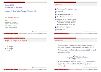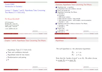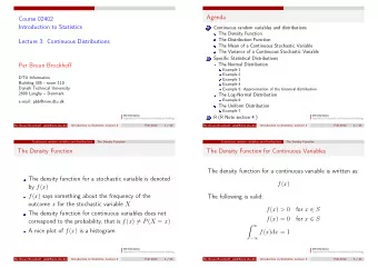
Overview Course 02402 Introduction to Statistics 1 Introduction to - PowerPoint PPT Presentation
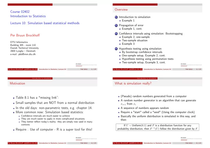
Overview Course 02402 Introduction to Statistics 1 Introduction to simulation Example 1 Lecture 10: Simulation based statistical methods 2 Propagation of error Example 1, cont. 3 Confidence intervals using simulation: Bootstrapping Per Bruun
Overview Course 02402 Introduction to Statistics 1 Introduction to simulation Example 1 Lecture 10: Simulation based statistical methods 2 Propagation of error Example 1, cont. 3 Confidence intervals using simulation: Bootstrapping Per Bruun Brockhoff Example 2, one-sample Two-sample situation DTU Informatics Example 3 Building 305 - room 110 Danish Technical University 4 Hypothesis testing using simulation 2800 Lyngby – Denmark By bootstrap confidence intervals e-mail: pbb@imm.dtu.dk One-sample setup, Example 2, cont. Hypothesis testing using permutation tests Two-sample setup, Example 3, cont. Per Bruun Brockhoff (pbb@imm.dtu.dk) Introduction to Statistics, Lecture 10 Fall 2012 1 / 27 Per Bruun Brockhoff (pbb@imm.dtu.dk) Introduction to Statistics, Lecture 10 Fall 2012 2 / 27 Introduction to simulation Introduction to simulation Motivation What is simulation really? (Pseudo) random numbers generated from a computer Table 8.1 has a "missing link”: A random number generator is an algorithm that can generate Small samples that are NOT from a normal distribution x i +1 from x i In the old days: non-parametric tests, e.g. chapter 14. A sequence of numbers appears random More common now: Simulation based statistics: Require a "start" called a "seed" (Using the computer clock) Confidence intervals are much easier to achieve Basically the uniform distribution is simulated in this way, and They are much easier to apply in more complicated situations then: They better reflect today’s reality: they are simply now used in many contexts If U ∼ Uniform (0 . 1) and F is a distribution function for any probability distribution, then F − 1 ( U ) follow the distribution given by F Require : Use of computer - R is a super tool for this! Per Bruun Brockhoff (pbb@imm.dtu.dk) Introduction to Statistics, Lecture 10 Fall 2012 4 / 27 Per Bruun Brockhoff (pbb@imm.dtu.dk) Introduction to Statistics, Lecture 10 Fall 2012 5 / 27
Introduction to simulation Introduction to simulation Example 1 In practice in R Example 1 A company produces rectangular plates. The length of plates (in The following (02402 relevant) distributions are ready for simulation: meters), X is assumed to follow a normal distribution N (2 , 0 . 1 2 ) and Binomial distribution the width of the plates (in meters), Y are assumed to follow a normal rbinom distribution N (3 , 0 . 2 2 ) . We are interested in the area of the plates Poisson distribution rpois The hypergeometric distribution which of course is given by A = XY . rhyper normal distribution rnorm What is the mean area? log-normal distributions rlnorm What is the standard deviation in the areas from plate to plate? exponential rexp how often such plates have an area that differ by more than The uniform distribution runif 0 . 1 m 2 from the targeted 6 m 2 ? t-distribution rt The probability of other events? χ 2 -distribution rchisq F distribution rf Generally: what is the probability distribution of the random variable A Per Bruun Brockhoff (pbb@imm.dtu.dk) Introduction to Statistics, Lecture 10 Fall 2012 6 / 27 Per Bruun Brockhoff (pbb@imm.dtu.dk) Introduction to Statistics, Lecture 10 Fall 2012 7 / 27 Introduction to simulation Example 1 Propagation of error Example 1, solution in R Propagation of error Must be able to find: σ 2 f ( X 1 ,...,X n ) = Var ( f ( X 1 , . . . , X n )) Result: We allready know: Code: > mean(A) k=10000 n n [1] 5.999061 � � σ 2 a 2 i σ 2 f ( X 1 ,...,X n ) = i , if f ( X 1 , . . . , X n ) = X=rnorm(k,2,0.1) a i X i > sd(A) Y=rnorm(k,3,0.2) i =1 i =1 A=X*Y [1] 0.5030009 New rule for non-linear funktions: mean(A) > sum(abs(A- sd(A) � ∂f n � 2 sum(abs(A-6)>0.1)/k 6)>0.1)/k � σ 2 σ 2 f ( X 1 ,...,X n ) ≈ i ∂X i [1] 0.8462 i =1 Per Bruun Brockhoff (pbb@imm.dtu.dk) Introduction to Statistics, Lecture 10 Fall 2012 8 / 27 Per Bruun Brockhoff (pbb@imm.dtu.dk) Introduction to Statistics, Lecture 10 Fall 2012 10 / 27
Propagation of error Propagation of error Example 1, cont. Propagation of error Example 1, cont. We already used the simulation method in the first part of the example. Given two specific measurements of X and Y , X = 2 . 05 m and y = 2 . 99 m . What is the variance of A = 2 . 05 × 2 . 99 = 6.13 Or by simulation: using the error propagation law? Simulate k outcomes of all n measurements as i ) : X ( j ) N ( X i , σ 2 i , j = 1 . . . , k Calculate the standard deviation directly as the observed standard deviation of the k values for f : � � k i =1 ( f j − ¯ 1 f ) 2 σ f ( X 1 ,...,X n ) = k − 1 f j = f ( X ( j ) 1 , . . . , X ( j ) n ) Per Bruun Brockhoff (pbb@imm.dtu.dk) Introduction to Statistics, Lecture 10 Fall 2012 11 / 27 Per Bruun Brockhoff (pbb@imm.dtu.dk) Introduction to Statistics, Lecture 10 Fall 2012 12 / 27 Propagation of error Example 1, cont. Confidence intervals using simulation: Bootstrapping Example 1, cont. Confidence intervals using simulation: Bootstrapping Actually one can deduce the variance of A theoretically, What to do with a small sample size ( n < 30) , and NO assumption of a normal distribution? − [ E ( XY )] 2 ( XY ) 2 � � Var ( XY ) = E Two possible solutions: E ( X 2 ) E ( Y 2 ) − E ( X ) 2 E ( Y ) 2 = Find/identify/assume a different and more suitable distribution for the 1 Var ( X ) + E ( X ) 2 � � Var ( Y ) + E ( Y ) 2 � − E ( X ) 2 E ( Y ) 2 � = population ("the system") Var ( X ) Var ( Y ) + Var ( X ) E ( Y ) 2 + Var ( Y ) E ( X ) 2 Do not assume any distribution whatsoever 2 = Bootstrapping exists in two versions: 0 . 1 2 × 0 . 2 2 + 0 . 1 2 × 3 2 + 0 . 2 2 × 2 2 = Parametric bootstrap: Simulate multiple samples from the assumed 1 = 0 . 0004 + 0 . 09 + 0 . 16 distribution. Non-parametric bootstrap: Simulate multiple samples directly from the 2 = 0 . 2504 data. Per Bruun Brockhoff (pbb@imm.dtu.dk) Introduction to Statistics, Lecture 10 Fall 2012 13 / 27 Per Bruun Brockhoff (pbb@imm.dtu.dk) Introduction to Statistics, Lecture 10 Fall 2012 15 / 27
Confidence intervals using simulation: Bootstrapping Confidence intervals using simulation: Bootstrapping Example 2, one-sample Non-parametric bootstrap for the one-sample situation Example 2, one-sample In a study women’s cigarette consumption before and after giving birth is explored. The following observations of the number of smoked cigarettes Data: x 1 , . . . , x n . per day were the results: 100(1 − α )% confidence interval for µ : before after before after Simulate k samples of size n by randomly sampling among the available data 8 5 13 15 (with replacement - large k , e.g. k > 1 . 000 ) 24 11 15 19 Calculate the average in each of the k samples ¯ x ∗ 1 , . . . , ¯ x ∗ k Calculate the 100 α/ 2% - and 100(1 − α/ 2)% percentiles for these 7 0 11 12 � � The confidence interval is: quantile 100 α/ 2% , quantile 100(1 − α/ 2)% 20 15 22 0 6 0 15 6 20 20 Per Bruun Brockhoff (pbb@imm.dtu.dk) Introduction to Statistics, Lecture 10 Fall 2012 16 / 27 Per Bruun Brockhoff (pbb@imm.dtu.dk) Introduction to Statistics, Lecture 10 Fall 2012 17 / 27 Confidence intervals using simulation: Bootstrapping Example 2, one-sample Confidence intervals using simulation: Bootstrapping Two-sample situation Example 2, solution in R Two-sample situation Data: Data: x 1 , . . . , x n 1 and y 1 , . . . , y n 2 x1=c(8,24,7,20,6,20,13,15,11,22,15) 100(1 − α )% confidence interval for µ 1 − µ 2 : x2=c(5,11,0,15,0,20,15,19,12,0,6) dif=x1-x2 Simulate k sets of 2 samples of size n 1 and n 2 R-Method 1: by sampling randomly from the respective groups k=10000 (with replacement - large k , eg. k > 1 . 000 ) mysamples = replicate(k, sample(dif, replace = TRUE)) Calculate the difference between the averages for mymeans = apply(mysamples, 2, mean) each of the k sample pairs: ¯ x ∗ 1 − ¯ y ∗ 1 , . . . , ¯ x ∗ k − ¯ y ∗ k quantile(mymeans,c(0.025,0.975)) Calculate the 100 α/ 2% - and 100(1 − α/ 2)% percentiles for these � � R-Method 2: (First install the package "bootstrap") The confidence interval is: quantile 100 α/ 2% , quantile 100(1 − α/ 2)% library(bootstrap) quantile(bootstrap(dif,k,mean)$thetastar,c(0.025,0.975)) Per Bruun Brockhoff (pbb@imm.dtu.dk) Introduction to Statistics, Lecture 10 Fall 2012 18 / 27 Per Bruun Brockhoff (pbb@imm.dtu.dk) Introduction to Statistics, Lecture 10 Fall 2012 19 / 27
Recommend
More recommend
Explore More Topics
Stay informed with curated content and fresh updates.
