Random Variables Will Perkins January 11, 2013 Random Variables - PowerPoint PPT Presentation

Random Variables Will Perkins January 11, 2013

Random Variables If a probability model describes an experiment, a random variable is a measurement - a number associated with each outcome of the experiment. A single experiment can involve multiple measurements related in many possible ways.

Measurable Functions Definition A function f : ( X , F ) → ( R , B ) is measurable if f − 1 ( B ) ∈ F for every B ∈ B . Fact: If B is the Borel σ -field then it is enough to check f − 1 (( −∞ , t ]) for all t .

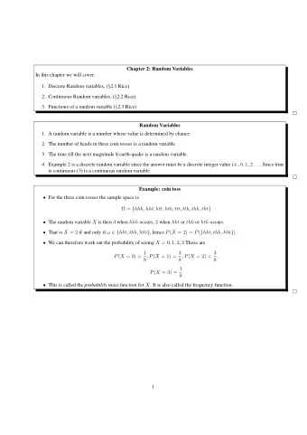
Random Variables Definition A random variable on a probability space ( X , F , P ) is a measurable function X : X → R . Examples: Flip a coin ten times, X = number of heads. Throw a dart at a dart board, X = distance from center. Throw a dart at a dartboard, X = 1 if bullseye, 0 otherwise. [This is called an indicator random variable] Throw a dart at the dartboard. X = 0 if a bullseye, distance from the bullseye otherwise.

Distribution Functions Definition The distribution function of a random variable X is the function F ( t ) = P [ X ≤ t ] Properties of distribution functions: 1 Every random variable has a distribution function. 2 Distribution functions are right-continuous and non-decreasing. 3 lim t →−∞ F ( t ) = 0 4 lim t →∞ F ( t ) = 1 5 Every such function is the distribution function of some random variable

Discrete Random Variables Definition A random variable X is discrete if there exists real numbers x 1 , x 2 , . . . so that ∞ � Pr[ X = x i ] = 1 i =1 The function f ( x ) = Pr[ X = x ] is called the probability mass function of X .

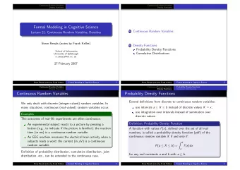
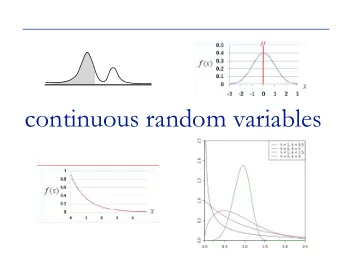
Continuous Random Variables Definition A random variable X is continuous if there is a function f ( x ) : R → R + so that � t Pr[ X ≤ t ] = f ( x ) dx −∞ f ( x ) is the density function for X . Note: there are random variabes which are neither continuous nor discrete. But every random variable has a distribution function.

Distributions Fact: Every random variable on (Ω , F , P ) induces a measure on ( R , B ). Proof: 1 Define µ X ( E ) = P ( X ∈ E ). 2 µ X ( R ) = 1, µ ( ∅ ) = 0. 3 Let E = ∪ ∞ i =1 E i with E i ∩ E j = ∅ . Then � µ X ( E ) = Pr( X ∈ ∪ E i ) = Pr( X ∈ E i ) i by the defintion of a function. µ X is the distribution of X (a measure on R ). Distributions are in 1-1 correspondence with distribution functions.

Examples: Discrete Some important discrete distributions: 1 Bernoulli(p). µ (1) = p , µ (0) = 1 − p . A biased coin flip. p k (1 − p ) n − k for 0 ≤ k ≤ n . � n 2 Binomial(n,p). µ ( k ) = � k Number of heads in n flips of a biased coin. 3 Geometric(p). µ ( k ) = p (1 − p ) k − 1 for k ≥ 1. Number of flips of a biased coin to get a head. 4 Poisson( λ ). µ ( k ) = e − λ λ k for k ≥ 0. The distribution of ‘rare k ! events’. 5 Discrete uniform(n). µ ( k ) = 1 n for k = 1 , . . . n .

Examples: Continuous Some important continuous distributions: 1 1 Uniform( a , b ). f ( x ) = b − a on [ a , b ]. 2 Exponential( λ ). f ( x ) = λ e − λ x on [0 , ∞ ). Distribution of waiting times. 2 πσ 2 e − ( x − µ ) 2 / 2 σ 2 on R . 3 Normal (Gaussian)( µ, σ 2 ). f ( x ) = 1 √ 2 π e − x 2 / 2 . Central Limit 1 Standard Normal (0,1): f ( x ) = √ Theorem. 4 Chi square(k). Sum of the sqares of k independent standard normals. Important in statistics.

Distribution functions and densities If X is a continuous rv, then f X ( x ) = F ′ X ( x ) Why? Fundamental Theorem of Calculus. � x F ( x ) = Pr[ X ≤ t ] = f ( t ) dt −∞

Multiple Measurements Most of what is interesting in probability deals with multiple random variables defined on the same probability space. Think of this as multiple, possibly related, measurements in the same experiment.

Random Vectors Definition Random Vector A random vector { X i } i ∈ I on (Ω , F , P ) is a collection of measurable functions X i on (Ω , F ). Definition Joint Distribution Function The joint distribution function of a random vector ( X 1 , X 2 , . . . X n ) is a function F : R n → [0 , 1] defined by: F ( t 1 , . . . t n ) = Pr[ X 1 ≤ t 1 ∩ X 2 ≤ t t ∩ · · · ∩ X n ≤ t n ]

Say X and Y are two random variables defined on the same probability space. Then ( X , Y ) is a random vector with a joint distribution (a measure on R 2 ). X and Y still have their own distributions (each measures on R ). These are called the marginal distributions of X and Y respectively. If you know the marginal distributions can you calculate the joint distribution? If you know the joint distribution can you calculate the marginal distributions?

Some Properties of Joint Distribution Functions 1 lim t 1 , t 2 →−∞ F X , Y ( t 1 , t 2 ) = 0 2 lim t 1 , t 2 →∞ F X , Y ( t 1 , t 2 ) = 1 3 lim t 1 →∞ F X , Y ( t 1 , t 2 ) = F Y ( t 2 ) 4 lim t 2 →∞ F X , Y ( t 1 , t 2 ) = F X ( t 1 ) 5 Discrete random vectors have joint probability mass functions, continuous random vectors have joint probability density functions.

Examples Flip two fair coins. Let X be the number of heads, Y the indicator rv that the first flip is a head. Find the marginal distributions of X and Y . Find the joint distribution of ( X , Y )

Examples Now let Z be the indicator that the first flip is a tail, and W the indicator that the second flip is a head. 1 Find the marginal distributions of Z , W and compare to Y . 2 Find the joint distribution of X , Y , Z , W 3 Find the joint distribution of Y , Z 4 Find the joint distribution of Y , W

Examples Let U ∼ Uniform [0 , 1] and let X be the indicator that U ≥ 1 / 2. 1 **What probability space are these random variables defined on?** 2 Find the marginal distributions. 3 Find the joint distributions.