P2 - Discrete Random Variables STAT 587 (Engineering) Iowa State - PowerPoint PPT Presentation
P2 - Discrete Random Variables STAT 587 (Engineering) Iowa State University August 21, 2020 Random variables Random variables If is the sample space of an experiment, a random variable X is a function X ( ) : R . Idea : If the
P2 - Discrete Random Variables STAT 587 (Engineering) Iowa State University August 21, 2020
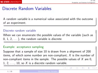
Random variables Random variables If Ω is the sample space of an experiment, a random variable X is a function X ( ω ) : Ω �→ R . Idea : If the value of a numerical variable depends on the outcome of an experiment, we call the variable a random variable . Examples of random variables from rolling two 6-sided dice: Sum of the two dice Indicator of the sum being greater than 5 We will use an upper case Roman letter (late in the alphabet) to indicate a random variable and a lower case Roman letter to indicate a realized value of the random variable.
Random variables 8 bit example Suppose, 8 bits are sent through a communication channel. Each bit has a certain probability to be received incorrectly. We are interested in the number of bits that are received incorrectly. Let X be the number of incorrect bits received. The possible values for X are { 0 , 1 , 2 , 3 , 4 , 5 , 6 , 7 , 8 } . Example events: No incorrect bits received: { X = 0 } . At least one incorrect bit received: { X ≥ 1 } . Exactly two incorrect bits received: { X = 2 } . Between two and seven (inclusive) incorrect bits received: { 2 ≤ X ≤ 7 } .
Random variables Range Range/image of random variables The range (or image) of a random variable X is defined as Range ( X ) := { x : x = X ( ω ) for some ω ∈ Ω } If the range is finite or countably infinite, we have a discrete random variable. If the range is uncountably infinite, we have a continuous random variable. Examples: Put a hard drive into service, measure Y = “time until the first major failure” and thus Range ( Y ) = (0 , ∞ ) . Range of Y is an interval (uncountable range), so Y is a continuous random variable. Communication channel: X = “# of incorrectly received bits out of 8 bits sent” with Range ( X ) = { 0 , 1 , 2 , 3 , 4 , 5 , 6 , 7 , 8 } . Range of X is a finite set, so X is a discrete random variable. Communication channel: Z = “# of incorrectly received bits in 10 minutes” with Range ( Z ) = { 0 , 1 , . . . } . Range of Z is a countably infinite set, so Z is a discrete random variable.
Discrete random variables Distribution Distribution The collection of all the probabilities related to X is the distribution of X . For a discrete random variable, the function p X ( x ) = P ( X = x ) is the probability mass function (pmf) and the cumulative distribution function (cdf) is � F X ( x ) = P ( X ≤ x ) = p X ( y ) . y ≤ x The set of non-zero probability values of X is called the support of the distribution f . This is the same as the range of X .
Discrete random variables Distribution Examples A probability mass function is valid if it defines a valid set of probabilities, i.e. they obey Kolmogorov’s axioms. Which of the following functions are a valid probability mass functions? x -3 -1 0 5 7 p X ( x ) 0.1 0.45 0.15 0.25 0.05 -1 0 1.5 3 4.5 y p Y ( y ) 0.1 0.45 0.25 -0.05 0.25 z 0 1 3 5 7 p Z ( z ) 0.22 0.18 0.24 0.17 0.18
Discrete random variables Die rolling Rolling a fair 6-sided die Let Y be the number of pips on the upturned face of a die. The support of Y is { 1 , 2 , 3 , 4 , 5 , 6 } . If we believe the die has equal probability for each face, then image, pmf, and cdf for Y are y 1 2 3 4 5 6 p Y ( y ) = P ( Y = y ) 1 1 1 1 1 1 6 6 6 6 6 6 F Y ( y ) = P ( Y ≤ y ) 1 2 3 4 5 6 6 6 6 6 6 6
Discrete random variables Dragonwood Dragonwood Dragonwood has 6-sided dice with the following # on the 6 sides: { 1 , 2 , 2 , 3 , 3 , 4 } . What is the support, pmf, and cdf for the sum of the upturned numbers when rolling 3 Dragonwood dice? # Three dice die = c(1,2,2,3,3,4) rolls = expand.grid(die1 = die, die2 = die, die3 = die) sum = rowSums(rolls); tsum = table(sum) dragonwood3 = data.frame(x = round(as.numeric(names(tsum)),0), pmf = round(as.numeric(table(sum)/length(sum)),3)) %>% mutate(cdf = cumsum(pmf)) t(dragonwood3) [,1] [,2] [,3] [,4] [,5] [,6] [,7] [,8] [,9] [,10] x 3.000 4.000 5.000 6.000 7.000 8.000 9.000 10.000 11.000 12.000 pmf 0.005 0.028 0.083 0.162 0.222 0.222 0.162 0.083 0.028 0.005 cdf 0.005 0.033 0.116 0.278 0.500 0.722 0.884 0.967 0.995 1.000
Discrete random variables Dragonwood Dragonwood - pmf and cdf 1.00 1.00 0.75 0.75 pmf cdf 0.50 0.50 0.25 0.25 0.00 0.00 3 4 5 6 7 8 9 10 11 12 3 4 5 6 7 8 9 10 11 12 x x
Discrete random variables Dragonwood Properties of pmf and cdf Properties of probability mass function p X ( x ) = P ( X = x ) : 0 ≤ p X ( x ) ≤ 1 for all x ∈ R . � x ∈ S p X ( x ) = 1 where S is the support. Properties of cumulative distribution function F X ( x ) : 0 ≤ F X ( x ) ≤ 1 for all x ∈ R F X is nondecreasing, (i.e. if x 1 ≤ x 2 then F X ( x 1 ) ≤ F X ( x 2 ) .) lim x →−∞ F X ( x ) = 0 and lim x →∞ F X ( x ) = 1 . F X ( x ) is right continuous with respect to x
Discrete random variables Dragonwood Dragonwood (cont.) In Dragonwood, you capture monsters by rolling a sum equal to or greater than its defense. Suppose you can roll 3 dice and the following monsters are available to be captured: Spooky Spiders worth 1 victory point with a defense of 3. Hungry Bear worth 3 victory points with a defense of 7. Grumpy Troll worth 4 victory points with a defense of 9. Which monster should you attack?
Discrete random variables Dragonwood Dragonwood (cont.) Calculate the probability by computing one minus the cdf evaluated at “defense minus 1”. Let X be the sum of the number on 3 Dragonwood dice. Then P ( X ≥ 3) = 1 − P ( X ≤ 2) = 1 P ( X ≥ 7) = 1 − P ( X ≤ 6) = 0 . 722 . P ( X ≥ 9) = 1 − P ( X ≤ 8) = 0 . 278 . If we multiply the probability by the number of victory points, then we have the “expected points”: 1 × P ( X ≥ 3) = 1 3 × P ( X ≥ 7) = 2 . 17 . 4 × P ( X ≥ 9) = 1 . 11 .
Discrete random variables Expectation Expectation Let X be a random variable and h be some function. The expected value of a function of a (discrete) random variable is � E [ h ( X )] = h ( x i ) · p X ( x i ) . i Intuition: Expected values are weighted averages of the possible values weighted by their probability. If h ( x ) = x , then � E [ X ] = x i · p X ( x i ) i and we call this the expectation of X and commonly use the symbol µ for the expectation.
Discrete random variables Expectation Dragonwood (cont.) What is the expectation of the sum of 3 Dragonwood dice? expectation = with(dragonwood3, sum(x*pmf)) expectation [1] 7.5 The expectation can be thought of as the center of mass if we place mass p X ( x ) at corresponding points x . 0.20 0.15 y 0.10 0.05 0.00 3 4 5 6 7 8 9 10 11 12 x
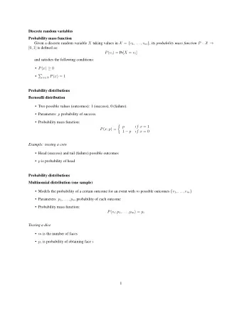
Discrete random variables Expectation Biased coin Suppose we have a biased coin represented by the following pmf: y 0 1 p Y ( y ) 1 − p p What is the expected value? If p = 0 . 9 , 0.75 0.50 pmf 0.25 0.00 0 1 y
Discrete random variables Properties of expectations Properties of expectations Let X and Y be random variables and a , b , and c be constants. Then E [ aX + bY + c ] = aE [ X ] + bE [ Y ] + c. In particular E [ X + Y ] = E [ X ] + E [ Y ] , E [ aX ] = aE [ X ] , and E [ c ] = c .
Discrete random variables Properties of expectations Dragonwood (cont.) Enhancement cards in Dragonwood allow you to improve your rolls. Here are two enhancement cards: Cloak of Darkness adds 2 points to all capture attempts and Friendly Bunny allows you (once) to roll an extra die. What is the expected attack roll total if you had 3 Dragonwood dice, the Cloak of Darkness, and are using the Friendly Bunny? Let X be the sum of 3 Dragonwood dice (we know E [ X ] = 7 . 5 ), Y be the sum of 1 Dragonwood die which has E [ Y ] = 2 . 5 . Then the attack roll total is X + Y + 2 and the expected attack roll total is E [ X + Y + 2] = E [ X ] + E [ Y ] + 2 = 7 . 5 + 2 . 5 + 2 = 12 .
Discrete random variables Variance Variance The variance of a random variable is defined as the expected squared deviation from the mean. For discrete random variables, variance is ( x i − µ ) 2 · p X ( x i ) � V ar [ X ] = E [( X − µ ) 2 ] = i where µ = E [ X ] . The symbol σ 2 is commonly used for the variance. The variance is analogous to moment of intertia in classical mechanics. The standard deviation (sd) is the positive square root of the variance: � SD [ X ] = V ar [ X ] . The symbol σ is commonly used for sd.
Discrete random variables Variance Properties of variance Two discrete random variables X and Y are independent if p X,Y ( x, y ) = p X ( x ) p Y ( y ) . If X and Y are independent, and a , b , and c are constants, then V ar [ aX + bY + c ] = a 2 V ar [ X ] + b 2 V ar [ Y ] . Special cases: V ar [ c ] = 0 V ar [ aX ] = a 2 V ar [ X ] V ar [ X + Y ] = V ar [ X ] + V ar [ Y ] (if X and Y are independent)
Discrete random variables Variance Dragonwood (cont.) What is the variance for the sum of the 3 Dragonwood dice? variance = with(dragonwood3, sum((x-expectation)^2*pmf)) variance [1] 2.766 What is the standard deviation for the sum of the pips on 3 Dragonwood dice? sqrt(variance) [1] 1.66313
Discrete random variables Variance Biased coin Suppose we have a biased coin represented by the following pmf: 0 1 y p Y ( y ) 1 − p p What is the variance? 1. E [ Y ] = p 2. V ar [ y ] = (0 − p ) 2 (1 − p ) + (1 − p ) 2 × p = p − p 2 = p (1 − p ) When is this variance maximized? 0.20 variance 0.10 0.00 0.0 0.2 0.4 0.6 0.8 1.0 y
Recommend
More recommend
Explore More Topics
Stay informed with curated content and fresh updates.
