Lecture 7 The Five Basic Discrete Random Variables In this lecture - PowerPoint PPT Presentation

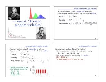
Lecture 7 The Five Basic Discrete Random Variables In this lecture we define and study the five basic discrete random variables. 0/ 26

The Five Basic Discrete Random Variables 1 Binomial 2 Hypergeometric 3 Geometric 4 Negative Binomial 5 Poisson Remark On the handout “The basic probability distributions” there are six distributions. I did not list the Bernoulli distribution above because it is too simple. In this lecture we will do 1. and 2. above. 1/ 26 Lecture 7The Five Basic Discrete Random Variables

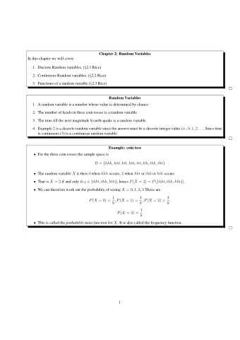
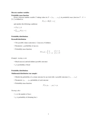
The Binomial Distribution Suppose we have a Bernoulli experiment with P ( S ) = P , for example, a weighted coin with P ( H ) = p . As usual we put q = 1 − p . Repeat the experiment (flip the coin). Let X = ♯ of successes ( ♯ of heads). We want to compute the probability distribution of X . Note, we did the special case n = 3 in Lecture 6, pages 4 and 5. 2/ 26 Lecture 7The Five Basic Discrete Random Variables

Clearly the set of possible values for X is 0 , 1 , 2 , 3 , . . . , n . Also P ( X = 0 ) = P ( TT T ) = qq . . . q = q n Explanation Here we assume the outcomes of each of the repeated experiments are independent so P (( T on 1 st ) ∩ ( T on 2 nd ) ∩ · · · ∩ ( T on n -th ) P ( T on 1 st ) P ( T on 2 rd ) . . . P ( T on n -th ) q q . . . q = q n Note T on 2 nd means T on 2 nd with no other information so P ( T on 2 nd ) = q . 3/ 26 Lecture 7The Five Basic Discrete Random Variables

Also P ( X = n ) = P ( HH . . . H ) = p n Now we have to work What is P ( X = 1 )? Another standard mistake The events ( X = 1 ) and HTT . . . T are NOT equal. � ������ �� ������ � n − 1 Why - the head doesn’t have to come on the first toss So in fact ( X = 1 ) = ( HTT . . . T ) ∪ ( THT . . . T ) ∪ · · · ∪ ( TTT . . . TH ) 4/ 26 Lecture 7The Five Basic Discrete Random Variables

All of the n events on the right have the same probability namely pq n − 1 and they are mutually exclusive. There are n of them so P ( X = 1 ) = npq n − 1 Similarly P ( X = n − 1 ) = npq n − 1 (exchange H and T above) 5/ 26 Lecture 7The Five Basic Discrete Random Variables

The general formula Now we want P ( X = k ) First we note ) = p k q n − k P ( H . . . H TT . . . T � �� �� �� � � ��� �� ��� � k n − k But again the heads don’t have to come first. So we need to (1) Count all the words of length n in H and T that involve k H ’s and n − k T ’s. (2) Multiply the number in (1) by p k q n − k . 6/ 26 Lecture 7The Five Basic Discrete Random Variables

So how do we solve 1. Think of filling n slot’s with k H ’s and n − k T ’s � ���������������������� �� ���������������������� � Main Point Once you decide where the k H ’s go you have no choice with the T ’s. They have to go in the remaining n − k slots. So choose the k -slots when the heads go. So we have to make a choose of k � n � things from n things so . k 7/ 26 Lecture 7The Five Basic Discrete Random Variables

So, � n � p k q n − k P ( X = k ) = k So we have motivated the following definition. Definition A discrete random variable X is said to have binomial distribution with parameters n and p (abbreviated X ∼ Bin ( n , p ) ) If X takes values 0 , 1 , 2 , . . . , n and � n � p k q n − k , 0 ≤ k ≤ n . P ( X = k ) = (*) k 8/ 26 Lecture 7The Five Basic Discrete Random Variables

Remark The text uses x instead of k for the independent (i.e., input) variable. So in the text this would be written � n � p x q n − x P ( X = x ) = x I like to save x for the variable case of continuous random variables however I will sometimes use x in the discrete case too. Finally we may write � n � p k q n − k , 0 ≤ k ≤ n p ( k ) = (**) k The text uses b ( · , n , p ) for p ( · ) so would write for (**) � n � p k q n − k b ( k , n , p ) = k 9/ 26 Lecture 7The Five Basic Discrete Random Variables

The Expected Value and Variance of a Binomial Random Variable Proposition Suppose X ∼ Bin ( n , p ) . Then E ( X ) = np and V ( X ) = npq so σ = standard deviation = √ npq. Remark The formula for E ( X ) is what you might expect. If you toss a fair coin 100 times � 1 � the E ( X ) = expected number of heads np = ( 100 ) = 50 . 2 However if you toss it 51 times then E ( X ) = 51 2 - not what you “expect”. 10/ 26 Lecture 7The Five Basic Discrete Random Variables

Using the binomial tables Table A1 in the text pg. A2,A3,A4 tabulate the cdf B ( x , n , p ) = P ( X ≤ x ) for n = 5 , 10 , 15 , 20 , 25 and selected values of p . Example (3.32) Suppose that 20% of all copies of a particular text book fail a certain binding strength text. Let X denote the number among 15 randomly selected copies that fail the test. Find P ( 4 ≤ X ≤ 7 ) . 11/ 26 Lecture 7The Five Basic Discrete Random Variables

Solution X ∼ Bin ( 15 , . 2 ) . We want to compute P ( 4 ≤ X ≤ 7 ) using the table on page 664. So how to we write P ( 4 ≤ X ≤ 7 ) in terms of terms of the form P ( X ≤ a ) 4 6 7 5 3 In the figure P ( X ≤ 3 ) is the region to the left of the left-most arc and P ( X ≤ 7 ) is the region to the left of the right-most arc. Answer ( ♯ ) P ( 4 ≤ X ≤ 7 ) = P ( X ≤ 7 ) − P ( X ≤ 3 ) So P ( 4 ≤ X ≤ 7 ) = B ( 7 , . 15 , . 2 ) − B ( 3 , . 15 , . 2 ) from table = . 996 − . 648 N.B. Understand ( ♯ ) . This the key using computers and statistical calculators to compute. 12/ 26 Lecture 7The Five Basic Discrete Random Variables

The hypergeometric distribution Example chips black chips white chips Consider an urn containing N chips of which M are black and L = N − M are white. Suppose we remove n chips without replacement so n ≤ N. In the figure there are 3 black chips and 2 white chips so in the picture N = 5 , M = 3 and L = 2 . Define a random variable X by X = ♯ of black chips we get. 13/ 26 Lecture 7The Five Basic Discrete Random Variables

Find the probability distribution of X . Proposition �� L � M � k n − k P ( X = k ) = (*) � N � n if ( b ) max( 0 , n − L ) ≤ k � min( n , M ) � ������������������������������������ �� ������������������������������������ � This means k ≤ both n and M and both 0 and n − L ≤ k. These are the possible values of k, that is, if k doesn’t satisfy (b) then P ( X = k ) = 0 . 14/ 26 Lecture 7The Five Basic Discrete Random Variables

Proof of the formula (*) Suppose we first consider the special case where all the chips are black so P ( X = n ) . This is the same problem as the one of finding all hearts in bridge. black chip ←→ heart white chip ←→ non heart So we use the principle of restricted choise � M � n P ( X = n ) = � N � n This agrees with (*). 15/ 26 Lecture 7The Five Basic Discrete Random Variables

But (*) is harder because we have to consider the case where there are k < n black chips. So we have to choose n − k white chips as well. � M � So choose k black chips, there are ways, then for each such choice, choose k � L � n − k white chips, there are ways. n − k So   choices of exactly � M �� �   L       ♯  = k black chips   k n − k      in the n chips 16/ 26 Lecture 7The Five Basic Discrete Random Variables

� N � Clearly there are ways of choosing n chips from N chips so (*) follows. n Definition If X is a discrete random variable with pmf defined by the formula in the previous Proposition then X is said to have hyper geometric distribution with parameters n, M, N. In the text the pmf is denoted h ( x ; n , M , N ) . 17/ 26 Lecture 7The Five Basic Discrete Random Variables

What about the conditions max( 0 , n − L ) ≤ k ≤ min( n , M ) (b) This really means k ≤ both n and M (b 1 ) and k ≥ both 0 and n − L (b 2 ) (b 1 ) says k ≤ n we can’t choose more then n ←→ black chips because we are only choosing n chips in total k ≤ M because there are only M black ←→ chips to choose from (b 2 ) k ≥ 0 is obvious and k ≥ n − L follows because k = n − L 18/ 26 Lecture 7The Five Basic Discrete Random Variables

So the above three inequalities are necessary. At first glance they look sufficient because if k satisfies the above three inequalities you can certainly go ahead and choose k black chips. But what about the white chips? We aren’t done yet, you have to choose n − k white chips and there are only L white chips available so if n − k > L we are sun k . So we must have n − k ≤ L ⇔ k ≥ n − L This is the second inequality of (b 2 ). If it is satisfied we can go ahead and choose the n − k white chips so the inequalities in (b) are necessary and sufficient. 19/ 26 Lecture 7The Five Basic Discrete Random Variables

Proposition Suppose X has hypergeometric distribution with parameters n, M, N. Then (i) E ( X ) = nM N � N − n � � � nM 1 − M (ii) V ( X ) = N − 1 N N If you put p = M the probability of getting N = a black chip on the first draw then we may rewrite the above formulas as reminiscent  E ( X ) = np   of the � N − n �   V ( X ) =  npq binomial    N − 1 distribution 20/ 26 Lecture 7The Five Basic Discrete Random Variables