Discrete Random Variables A random variable is a numerical value - PowerPoint PPT Presentation
ST 370 Probability and Statistics for Engineers Discrete Random Variables A random variable is a numerical value associated with the outcome of an experiment. Discrete random variable When we can enumerate the possible values of the variable
ST 370 Probability and Statistics for Engineers Discrete Random Variables A random variable is a numerical value associated with the outcome of an experiment. Discrete random variable When we can enumerate the possible values of the variable (such as 0, 1, 2, . . . ), the random variable is discrete . Example: acceptance sampling Suppose that a sample of size 10 is drawn from a shipment of 200 items, of which some number are non-compliant; X is the number of non-compliant items in the sample. The possible values of X are 0, 1, 2, . . . , 10, so X is a discrete random variable. 1 / 15 Discrete Random Variables
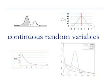
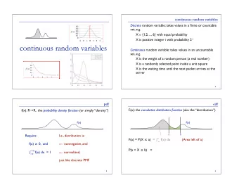
ST 370 Probability and Statistics for Engineers Continuous random variable When the variable takes values in an entire interval, the random variable is continuous . Example: flash unit recharge time Suppose that a cell phone camera flash is chosen randomly from a production line; the time X that it takes to recharge is a positive real number; X is a continuous random variable. Presumably, there is some lower bound a > 0 that is the shortest possible recharge time, and similarly some upper bound b < ∞ that is the longest possible recharge time; however, we usually do not know these values, and we would just say that the possible values of X are { x : 0 < x < ∞} . 2 / 15 Discrete Random Variables
ST 370 Probability and Statistics for Engineers Probability distribution The probability distribution of a random variable X is a description of the probabilities associated with the possible values of X . The representation of a probability distribution is different for discrete and continuous random variables. Probability mass function For a discrete random variable, the simplest representation is the probability mass function (pmf) f X ( x ) = P ( X = x ) where x is any possible value of X . 3 / 15 Discrete Random Variables Probability distribution
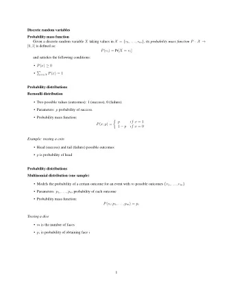
ST 370 Probability and Statistics for Engineers Example: acceptance sampling Suppose one item is chosen at random from a shipment of 200 items, of which 5 are non-compliant. Let � 1 if the item is non-compliant, X = 0 if the item is compliant. We could say that X is the number of non-compliant items seen. The probability mass function of X is � 0 . 975 x = 0 f X ( x ) = 0 . 025 x = 1 A random variable like X that takes only the values 0 and 1 is called a Bernoulli random variable. 4 / 15 Discrete Random Variables Probability distribution
ST 370 Probability and Statistics for Engineers Example: Dice Suppose you roll a fair die, and the number of spots showing is X . Then X is a discrete random variable with probability mass function f X ( x ) = 1 6 , x = 1 , 2 , 3 , 4 , 5 , 6 . Because the probability is the same for all the possible values of X , it is called the discrete uniform distribution. Properties of the probability mass function They are probabilities: f X ( x ) ≥ 0. They cover all possibilities: � x f X ( x ) = 1. 5 / 15 Discrete Random Variables Probability distribution
ST 370 Probability and Statistics for Engineers Cumulative distribution function As an alternative to the probability mass function, the probability distribution of a random variable X can be defined by its cumulative distribution function (cdf) F X ( x ) = P ( X ≤ x ) , −∞ < x < ∞ . In terms of the probability mass function: � F X ( x ) = f x ( x i ) , −∞ < x < ∞ . x i ≤ x F X ( · ) has a jump at each possible value x i of X , and the jump equals the corresponding probability f X ( x i ), so the probability mass function can be obtained from the cumulative distribution function. 6 / 15 Discrete Random Variables Cumulative distribution function
ST 370 Probability and Statistics for Engineers Example: acceptance sampling 0 x < 0 F X ( x ) = 0 . 975 0 ≤ x < 1 1 x ≥ 1 curve(pbinom(x, 1, .025), from = -1, to = 2) 7 / 15 Discrete Random Variables Cumulative distribution function
ST 370 Probability and Statistics for Engineers Example: dice 0 x < 1 1 / 6 1 ≤ x < 2 2 / 6 2 ≤ x < 3 F X ( x ) = . . . 1 x ≥ 6 curve(pmax(0, pmin(1, floor(x)/6)), from = 0, to = 7) 8 / 15 Discrete Random Variables Cumulative distribution function
ST 370 Probability and Statistics for Engineers Mean and Variance Mean value The mean value , or expected value, of a discrete random variable with probability mass function f X ( · ) is � µ X = E ( X ) = xf X ( x ) . x E ( X ) is a weighted average of the possible values of X , each weighted by the corresponding probability. The expected value E ( X ) is a typical value of the random variable X , in the same way that a sample mean ¯ x is a typical value of the sample x 1 , x 2 , . . . , x n . 9 / 15 Discrete Random Variables Mean and Variance
ST 370 Probability and Statistics for Engineers Example: acceptance sampling One item is chosen at random from a shipment of 200 items, of which 5 are non-compliant, and X is the number of non-compliant items seen: E ( X ) = 0 × f X (0) + 1 × f X (1) = 0 . 025 . For any Bernoulli random variable X , E ( X ) = P ( X = 1) . 10 / 15 Discrete Random Variables Mean and Variance
ST 370 Probability and Statistics for Engineers Example: Dice Suppose you roll a fair die, and the number of spots showing is X : E ( X ) = 1 × f X (1) + 2 × f X (2) + · · · + 6 × f X (6) = (1 + 2 + 3 + 4 + 5 + 6) / 6 = 3 . 5 . Note In these examples and in many others, the “expected” value is not one of the possible values of the random variable; this is not the paradox that it is sometimes made out to be! 11 / 15 Discrete Random Variables Mean and Variance
ST 370 Probability and Statistics for Engineers Variance Suppose that X is a random variable with expected value µ X . Then Y = ( X − µ X ) 2 is another random variable, and its expected value is � E ( Y ) = yf Y ( y ) y � ( x − µ X ) 2 f X ( x ) . = x 12 / 15 Discrete Random Variables Mean and Variance
ST 370 Probability and Statistics for Engineers The variance of X is E ( Y ) = E [( X − µ X ) 2 ]: σ 2 ( X − µ X ) 2 � � X = V ( X ) = E . The standard deviation of X is � σ 2 σ X = X . 13 / 15 Discrete Random Variables Mean and Variance
ST 370 Probability and Statistics for Engineers Example: acceptance sampling For any Bernoulli random variable X , µ X = P ( X = 1) = p , say , so X = (0 − p ) 2 × P ( X = 0) + (1 − p ) 2 × P ( X = 1) σ 2 = p 2 (1 − p ) + (1 − p ) 2 p = p (1 − p ) and � σ X = p (1 − p ) . 14 / 15 Discrete Random Variables Mean and Variance
ST 370 Probability and Statistics for Engineers Example: Dice ( x − 3 . 5) 2 ( x − 3 . 5) 2 f X ( x ) x x − 3 . 5 f X ( x ) 1 1 -2.5 6.25 1.0417 6 1 2 -1.5 2.25 0.3750 6 1 3 -0.5 0.25 0.0417 6 1 4 0.5 0.25 0.0417 6 1 5 1.5 2.25 0.3750 6 1 6 2.5 6.25 1.0417 6 Total: 2.9168 So σ 2 X = 2 . 917 and σ X = 1 . 708. 15 / 15 Discrete Random Variables Mean and Variance
Recommend
More recommend
Explore More Topics
Stay informed with curated content and fresh updates.
