Randome Variables and Expectation Example: Finding the k -Smallest - PowerPoint PPT Presentation
Randome Variables and Expectation Example: Finding the k -Smallest Element in an ordered set. Procedure Order( S , k ); Input: A set S , an integer k | S | = n . Output: The k smallest element in the set S . Example: Finding the k -Smallest
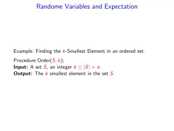
Randome Variables and Expectation Example: Finding the k -Smallest Element in an ordered set. Procedure Order( S , k ); Input: A set S , an integer k ≤ | S | = n . Output: The k smallest element in the set S .
Example: Finding the k -Smallest Element Procedure Order( S , k ); Input: A set S , an integer k ≤ | S | = n . Output: The k smallest element in the set S . 1 If | S | = k = 1 return S . 2 Choose a random element y uniformly from S . 3 Compare all elements of S to y . Let S 1 = { x ∈ S | x ≤ y } and S 2 = { x ∈ S | x > y } . 4 If k ≤ | S 1 | return Order( S 1 , k ) else return Order( S 2 , k − | S 1 | ). Theorem 1 The algorithm always returns the k-smallest element in S 2 The algorithm performs O ( n ) comparisons in expectation .
Random Variable Definition A random variable X on a sample space Ω is a real-valued function on Ω; that is, X : Ω → R . A discrete random variable is a random variable that takes on only a finite or countably infinite number of values. Discrete random variable X and real value a : the event “ X = a ” represents the set { s ∈ Ω : X ( s ) = a } . � Pr( X = a ) = Pr( s ) s ∈ Ω: X ( s )= a
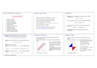
Independence Definition Two random variables X and Y are independent if and only if Pr(( X = x ) ∩ ( Y = y )) = Pr( X = x ) · Pr( Y = y ) for all values x and y . Similarly, random variables X 1 , X 2 , . . . X k are mutually independent if and only if for any subset I ⊆ [1 , k ] and any values x i , i ∈ I , �� � � Pr X i = x i = Pr( X i = x i ) . i ∈ I i ∈ I
Expectation Definition The expectation of a discrete random variable X , denoted by E [ X ], is given by � E [ X ] = i Pr( X = i ) , i where the summation is over all values in the range of X . The expectation is finite if � i | i | Pr( X = i ) converges; otherwise, the expectation is unbounded. The expectation (or mean or average) is a weighted sum over all possible values of the random variable.
Median Definition The median of a random variable X is a value m such Pr ( X < m ) ≤ 1 / 2 and Pr ( X > m ) < 1 / 2 .
Linearity of Expectation Theorem For any two random variables X and Y E [ X + Y ] = E [ X ] + E [ Y ] . Lemma For any constant c and discrete random variable X, E [ cX ] = c E [ X ] .
Example: Finding the k -Smallest Element Procedure Order( S , k ); Input: A set S , an integer k ≤ | S | = n . Output: The k smallest element in the set S . 1 If | S | = k = 1 return S . 2 Choose a random element y uniformly from S . 3 Compare all elements of S to y . Let S 1 = { x ∈ S | x ≤ y } and S 2 = { x ∈ S | x > y } . 4 If k ≤ | S 1 | return Order( S 1 , k ) else return Order( S 2 , k − | S 1 | ). Theorem 1 The algorithm always returns the k-smallest element in S 2 The algorithm performs O ( n ) comparisons in expectation .
Proof • We say that a call to Order( S , k ) was successful if the random element was in the middle 1 / 3 of the set S . A call is successful with probability 1 / 3. • After the i -th successful call the size of the set S is bounded by n (2 / 3) i . Thus, need at most log 3 / 2 n successful calls. • Let X be the total number of comparisons. Let T i be the number of iterations between the i -th successful call (included) and the i + 1-th (excluded): E [ X ] ≤ � log 3 / 2 n n (2 / 3) i E [ T i ]. i =0 • T i has a geometric distribution G (1 / 3).
The Geometric Distribution Definition A geometric random variable X with parameter p is given by the following probability distribution on n = 1 , 2 , . . . . Pr( X = n ) = (1 − p ) n − 1 p . Example: repeatedly draw independent Bernoulli random variables with parameter p > 0 until we get a 1. Let X be number of trials up to and including the first 1. Then X is a geometric random variable with parameter p .
Lemma Let X be a discrete random variable that takes on only non-negative integer values. Then ∞ � E [ X ] = Pr( X ≥ i ) . i =1 Proof. ∞ ∞ ∞ � � � Pr( X ≥ i ) = Pr( X = j ) i =1 i =1 j = i j ∞ � � = Pr( X = j ) j =1 i =1 ∞ � = j Pr( X = j ) = E [ X ] . j =1
For a geometric random variable X with parameter p , ∞ � (1 − p ) n − 1 p = (1 − p ) i − 1 . Pr( X ≥ i ) = n = i ∞ � E [ X ] = Pr( X ≥ i ) i =1 ∞ � (1 − p ) i − 1 = i =1 1 = 1 − (1 − p ) 1 = p
Proof • Let X be the total number of comparisons. • Let T i be the number of iterations between the i -th successful call (included) and the i + 1-th (excluded): • E [ X ] ≤ � log 3 / 2 n n (2 / 3) i E [ T i ]. i =0 • T i ∼ G (1 / 3), therefore E [ T i ] = 3. • Expected number of comparisons: log 3 / 2 n � j � 2 � E [ X ] ≤ 3 n ≤ 9 n . 3 j =0 Theorem 1 The algorithm always returns the k-smallest element in S 2 The algorithm performs O ( n ) comparisons in expectation . What is the probability space?
Finding the k -Smallest Element with no Randomization Procedure Det-Order( S , k ); Input: An array S , an integer k ≤ | S | = n . Output: The k smallest element in the set S . 1 If | S | = k = 1 return S . 2 Let y be the first element is S . 3 Compare all elements of S to y . Let S 1 = { x ∈ S | x ≤ y } and S 2 = { x ∈ S | x > y } . 4 If k ≤ | S 1 | return Det-Order( S 1 , k ) else return Det-Order( S 2 , k − | S 1 | ). Theorem The algorithm returns the k-smallest element in S and performs O ( n ) comparisons in expectation over all possible input permutations.
Randomized Algorithms: • Analysis is true for any input. • The sample space is the space of random choices made by the algorithm. • Repeated runs are independent. Probabilistic Analysis: • The sample space is the space of all possible inputs. • If the algorithm is deterministic repeated runs give the same output.
Algorithm classification A Monte Carlo Algorithm is a randomized algorithm that may produce an incorrect solution. For decision problems: A one-side error Monte Carlo algorithm errs only one one possible output, otherwise it is a two-side error algorithm. A Las Vegas algorithm is a randomized algorithm that always produces the correct output. In both types of algorithms the run-time is a random variable.
Expectation is not everything. . . Which algorithm do you prefer? 1 Algorithm I: takes 1 minute with probability 0 . 99, but with probability 0 . 01 takes an hour. 2 Algorithm II: takes 1 min with probability 1 / 2 and 3 minutes with probability 1 / 2.
Expectation is not everything. . . Which algorithm do you prefer? 1 Algorithm I: takes 1 minute with probability 0 . 99, but with probability 0 . 01 takes an hour. (Expected run-time 1 . 6.) 2 Algorithm II: takes 1 min with probability 1 / 2 and 3 minutes with probability 1 / 2. (Expected run-time 2.) In addition to expectation we need a bound on the probability that the run time of the algorithm deviates significantly from its expectation.
Bounding Deviation from Expectation Theorem [Markov Inequality] For any non-negative random variable X, and for all a > 0 , Pr ( X ≥ a ) ≤ E [ X ] . a Proof. � � E [ X ] = iPr ( X = i ) ≥ a Pr ( X = i ) = aPr ( X ≥ a ) . i ≥ a Example: The expected number of comparisons executed by the k -select algorithm was 9 n . The probability that it executes 18 n comparisons or more ≤ 9 n 18 n = 1 2 .
Variance Definition The variance of a random variable X is Var [ X ] = E [( X − E [ X ]) 2 ] = E [ X 2 ] − ( E [ X ]) 2 . Definition The standard deviation of a random variable X is � σ ( X ) = Var [ X ] .
Chebyshev’s Inequality Theorem For any random variable X, and any a > 0 , Pr ( | X − E [ X ] | ≥ a ) ≤ Var [ X ] . a 2 Proof. Pr ( | X − E [ X ] | ≥ a ) = Pr (( X − E [ X ]) 2 ≥ a 2 ) By Markov inequality Pr (( X − E [ X ]) 2 ≥ a 2 ) ≤ E [( X − E [ X ]) 2 ] a 2 = Var [ X ] a 2
Theorem For any random variable X and any a > 0 : Pr ( | X − E [ X ] | ≥ a σ [ X ]) ≤ 1 a 2 . Theorem For any random variable X and any ε > 0 : Var [ X ] Pr ( | X − E [ X ] | ≥ ε E [ X ]) ≤ ε 2 ( E [ X ]) 2 .
Theorem If X and Y are independent random variables E [ XY ] = E [ X ] · E [ Y ] . Proof. � � E [ XY ] = i · jPr (( X = i ) ∩ ( Y = j )) = i j � � ijPr ( X = i ) · Pr ( Y = j ) = i j � �� � . iPr ( X = i ) jPr ( Y = j ) i j
Theorem If X and Y are independent random variables Var [ X + Y ] = Var [ X ] + Var [ Y ] . Proof. Var [ X + Y ] = E [( X + Y − E [ X ] − E [ Y ]) 2 ] = E [( X − E [ X ]) 2 + ( Y − E [ Y ]) 2 + 2( X − E [ X ])( Y − E [ Y ])] = Var [ X ] + Var [ Y ] + 2 E [ X − E [ X ]] E [ Y − E [ Y ]] Since the random variables X − E [ X ] and Y − E [ Y ] are independent. But E [ X − E [ X ]] = E [ X ] − E [ X ] = 0 .
Bernoulli Trial Let X be a 0-1 random variable such that Pr ( X = 1) = p , Pr ( X = 0) = 1 − p . E [ X ] = 1 · p + 0 · (1 − p ) = p . Var [ X ] = p (1 − p ) 2 + (1 − p )(0 − p ) 2 = p (1 − p )(1 − p + p ) = p (1 − p ) .
A Binomial Random variable Consider a sequence of n independent Bernoulli trials X 1 , ...., X n . Let n � X = X i . i =1 X has a Binomial distribution X ∼ B ( n , p ). � n � p k (1 − p ) n − k . Pr ( X = k ) = k E [ X ] = np . Var [ X ] = np (1 − p ) .
Recommend
More recommend
Explore More Topics
Stay informed with curated content and fresh updates.
