CS70: Jean Walrand: Lecture 27. Expectation; Conditional - PowerPoint PPT Presentation

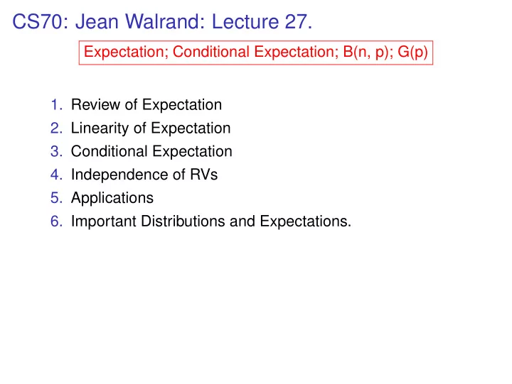
CS70: Jean Walrand: Lecture 27. Expectation; Conditional Expectation; B(n, p); G(p) 1. Review of Expectation 2. Linearity of Expectation 3. Conditional Expectation 4. Independence of RVs 5. Applications 6. Important Distributions and Expectations.

Expectation Recall: X : Ω → ℜ ; Pr [ X = a ];= Pr [ X − 1 ( a )] ; Definition: The expectation of a random variable X is E [ X ] = ∑ a × Pr [ X = a ] . a Indicator: Let A be an event. The random variable X defined by � 1 , if ω ∈ A X ( ω ) = 0 , if ω / ∈ A is called the indicator of the event A . Note that Pr [ X = 1 ] = Pr [ A ] and Pr [ X = 0 ] = 1 − Pr [ A ] . Hence, E [ X ] = 1 × Pr [ X = 1 ]+ 0 × Pr [ X = 0 ] = Pr [ A ] . The random variable X is sometimes written as 1 { ω ∈ A } or 1 A ( ω ) .

Linearity of Expectation Theorem: E [ X ] = ∑ X ( ω ) × Pr [ ω ] . ω Theorem: Expectation is linear E [ a 1 X 1 + ··· + a n X n ] = a 1 E [ X 1 ]+ ··· + a n E [ X n ] . Proof: E [ a 1 X 1 + ··· + a n X n ] = ∑ ( a 1 X 1 + ··· + a n X n )( ω ) Pr [ ω ] ω = ∑ ( a 1 X 1 ( ω )+ ··· + a n X n ( ω )) Pr [ ω ] ω = a 1 ∑ X 1 ( ω ) Pr [ ω ]+ ··· + a n ∑ X n ( ω ) Pr [ ω ] ω ω = a 1 E [ X 1 ]+ ··· + a n E [ X n ] .

Using Linearity - 1: Pips on dice Roll a die n times. X m = number of pips on roll m . X = X 1 + ··· + X n = total number of pips in n rolls. E [ X ] = E [ X 1 + ··· + X n ] = E [ X 1 ]+ ··· + E [ X n ] , by linearity = nE [ X 1 ] , because the X m have the same distribution Now, E [ X 1 ] = 1 × 1 6 + ··· + 6 × 1 6 = 6 × 7 × 1 6 = 7 2 . 2 Hence, E [ X ] = 7 n 2 .

Using Linearity - 2: Fixed point. Hand out assignments at random to n students. X = number of students that get their own assignment back. X = X 1 + ··· + X n where X m = 1 { student m gets his/her own assignment back } . One has E [ X ] = E [ X 1 + ··· + X n ] = E [ X 1 ]+ ··· + E [ X n ] , by linearity = nE [ X 1 ] , because all the X m have the same distribution = nPr [ X 1 = 1 ] , because X 1 is an indicator = n ( 1 / n ) , because student 1 is equally likely to get any one of the n assignments = 1 . Note that linearity holds even though the X m are not independent (whatever that means).

Using Linearity - 3: Binomial Distribution. Flip n coins with heads probability p . X - number of heads Binomial Distibution: Pr [ X = i ] , for each i . � n � p i ( 1 − p ) n − i . Pr [ X = i ] = i � n � E [ X ] = ∑ i × Pr [ X = i ] = ∑ p i ( 1 − p ) n − i . i × i i i Uh oh. ... Or... a better approach: Let � 1 if i th flip is heads X i = 0 otherwise E [ X i ] = 1 × Pr [“ heads ′′ ]+ 0 × Pr [“ tails ′′ ] = p . Moreover X = X 1 + ··· X n and E [ X ] = E [ X 1 ]+ E [ X 2 ]+ ··· E [ X n ] = n × E [ X i ]= np .

Conditional Expectation How do observations affect expectation? Example 1: Roll one die. You are told that the outcome X is at least 3. What is the expected value of X given that information? Given that X ≥ 3, we know that X is uniform in { 3 , 4 , 5 , 6 } . Hence, the mean value is 4 . 5. We write E [ X | X ≥ 3 ] = 4 . 5 . Similarly, we have E [ X | X < 3 ] = 1 . 5 because, given that X < 3, X is uniform in { 1 , 2 } . Note that E [ X | X ≥ 3 ] × Pr [ X ≥ 3 ]+ E [ X | X < 2 ] × Pr [ X < 2 ] = 4 . 5 × 4 6 + 1 . 5 × 2 6 = 3 + 0 . 5 = 3 . 5 = E [ X ] . Is this a coincidence?

Conditional Expectation How do observations affect expectation? Example 2: Roll two dice. You are told that the total number X of pips is at least 8. What is the expected value of X given that information? Recall the distribution of X : Pr [ X = 2 ] = Pr [ X = 12 ] = 1 / 36 , Pr [ X = 3 ] = Pr [ X = 11 ] = 2 / 36 ,... . Given that X ≥ 8, the distribution of X becomes { ( 8 , 5 / 15 ) , ( 9 , 4 / 15 ) , ( 10 , 3 / 15 ) , ( 11 , 2 / 15 ) , ( 12 , 1 / 15 ) } . For instance, Pr [ X = 8 | X ≥ 8 ] = Pr [ X = 8 ] Pr [ X ≥ 8 ] = 5 / 36 15 / 36 = 5 15 . Hence, E [ X | X ≥ 8 ] = 8 5 15 + 9 4 15 + 10 3 15 + 11 2 15 + 12 1 15 = 140 15 ≈ 9 . 33 .

Conditional Expectation How do observations affect expectation? Example 2: continued Roll two dice. You are told that the total number X of pips is less than 8. What is the expected value of X given that information? We find that E [ X | X < 8 ] = 2 1 21 + 3 3 21 + ··· + 7 6 21 = 112 21 ≈ 5 . 33 . Observe that E [ X | X ≥ 8 ] Pr [ X ≥ 8 ]+ E [ X | X < 8 ] Pr [ X < 8 ] = 9 . 33 × 15 36 + 5 . 3321 36 = 7 = E [ X ] . Coincidence? Probably not.

Conditional Probability Definition Let X be a RV and A an event. Then E [ X | A ] := ∑ a × Pr [ X = a | A ] . a It is easy (really) to see that 1 E [ X | A ] = ∑ Pr [ A ] ∑ X ( ω ) Pr [ ω | A ] = X ( ω ) Pr [ ω ] . ω ∈ A ω Theorem Conditional Expectation is linear E [ a 1 X 1 + ··· + a n X n | A ] = a 1 E [ X 1 | A ]+ ··· + a n E [ X n | A ] . Proof: E [ a 1 X 1 + ··· + a n X n | A ] = ∑ [ a 1 X 1 ( ω )+ ··· + a n X n ( ω )] Pr [ ω | A ] ω = a 1 ∑ X 1 ( ω ) Pr [ ω | A ]+ ··· + a n ∑ X n ( ω ) Pr [ ω | A ] ω ω = a 1 E [ X 1 | A ]+ ··· a n E [ X n | A ] .

Conditional Probability Theorem E [ X ] = E [ X | A ] Pr [ A ]+ E [ X | ¯ A ] Pr [¯ A ] . Proof The law of total probability says that Pr [ ω ] = Pr [ ω | A ] Pr [ A ]+ Pr [ ω | ¯ A ] Pr [¯ A ] . Hence, = ∑ E [ X ] X ( ω ) Pr [ ω ] ω = ∑ X ( ω ) Pr [ ω | ¯ A ] Pr [¯ X ( ω ) Pr [ ω | A ] Pr [ A ]+ ∑ A ] ω ω E [ X | A ] Pr [ A ]+ E [ X | ¯ A ] Pr [¯ = A ] .

Geometric Distribution Let’s flip a coin with Pr [ H ] = p until we get H . For instance: ω 1 = H , or ω 2 = T H , or ω 3 = T T H , or ω n = T T T T ··· T H . Note that Ω = { ω n , n = 1 , 2 ,... } . Let X be the number of flips until the first H . Then, X ( ω n ) = n . Also, Pr [ X = n ] = ( 1 − p ) n − 1 p , n ≥ 1 .

Geometric Distribution Pr [ X = n ] = ( 1 − p ) n − 1 p , n ≥ 1 .

Geometric Distribution Pr [ X = n ] = ( 1 − p ) n − 1 p , n ≥ 1 . Note that ∞ ∞ ∞ ∞ ( 1 − p ) n − 1 = p ( 1 − p ) n − 1 p = p ( 1 − p ) n . ∑ ∑ ∑ ∑ Pr [ X n ] = n = 1 n = 1 n = 1 n = 0 n = 0 a n = Now, if | a | < 1, then S := ∑ ∞ 1 1 − a . Indeed, 1 + a + a 2 + a 3 + ··· S = a + a 2 + a 3 + a 4 + ··· aS = 1 + a − a + a 2 − a 2 + ··· = 1 . ( 1 − a ) S = Hence, ∞ 1 ∑ Pr [ X n ] = p 1 − ( 1 − p ) = 1 . n = 1

Geometric Distribution: Expectation X = D G ( p ) , i.e., Pr [ X = n ] = ( 1 − p ) n − 1 p , n ≥ 1 . One has ∞ ∞ n ( 1 − p ) n − 1 p . ∑ ∑ E [ X ] = nPr [ X = n ] = n = 1 n = 1 Thus, p + 2 ( 1 − p ) p + 3 ( 1 − p ) 2 p + 4 ( 1 − p ) 3 p + ··· E [ X ] = ( 1 − p ) p + 2 ( 1 − p ) 2 p + 3 ( 1 − p ) 3 p + ··· ( 1 − p ) E [ X ] = p + ( 1 − p ) p + ( 1 − p ) 2 p + ( 1 − p ) 3 p + ··· pE [ X ] = by subtracting the previous two identities ∞ ∑ = Pr [ X = n ] = 1 . n = 1 Hence, E [ X ] = 1 p .

Geometric Distribution: Renewal Trick A different look at the algebra. We flip the coin once, and, if we get T , let ω be the following flips. Note that X ( H ω ) = 1 and X ( T ω ) = 1 + Y ( ω ) . Hence, = ∑ 1 × Pr [ H ω ]+ ∑ E [ X ] ( 1 + Y ( ω )) Pr [ T ω ] ω ω = ∑ pPr [ ω ]+ ∑ ( 1 + Y ( ω ))( 1 − p ) Pr [ ω ] ω ω = p +( 1 − p )( 1 + E [ Y ]) = 1 +( 1 − p ) E [ Y ] . But, E [ X ] = E [ Y ] . Thus, E [ X ] = 1 +( 1 − p ) E [ X ] , so that E [ X ] = 1 / p .

Geometric Distribution: Memoryless Let X be G ( p ) . Then, for n ≥ 0, Pr [ X > n ] = Pr [ first n flips are T ] = ( 1 − p ) n . Theorem Pr [ X > n + m | X > n ] = Pr [ X > m ] , m , n ≥ 0 . Proof: Pr [ X > n + m and X > n ] Pr [ X > n + m | X > n ] = Pr [ X > n ] Pr [ X > n + m ] = Pr [ X > n ] ( 1 − p ) n + m = ( 1 − p ) m = ( 1 − p ) n = Pr [ X > m ] .

Geometric Distribution: Memoryless - Interpretation Pr [ X > n + m | X > n ] = Pr [ X > m ] , m , n ≥ 0 . Pr [ X > n + m | X > n ] = Pr [ A | B ] = Pr [ A ] = Pr [ X > m ] . The coin is memoryless, therefore, so is X .

Geometric Distribution: Yet another look Theorem: For a r.v. X that takes the values { 0 , 1 , 2 ,... } , one has ∞ ∑ E [ X ] = Pr [ X ≥ i ] . i = 1 [See later for a proof.] If X = G ( p ) , then Pr [ X ≥ i ] = Pr [ X > i − 1 ] = ( 1 − p ) i − 1 . Hence, ∞ ∞ 1 − ( 1 − p ) = 1 1 ( 1 − p ) i − 1 = ( 1 − p ) i = ∑ ∑ E [ X ] = p . i = 1 i = 0

Expected Value of Integer RV Theorem: For a r.v. X that takes values in { 0 , 1 , 2 ,... } , one has ∞ ∑ E [ X ] = Pr [ X ≥ i ] . i = 1 Proof: One has ∞ ∑ E [ X ] = i × Pr [ X = i ] i = 1 ∞ ∑ = i { Pr [ X ≥ i ] − Pr [ X ≥ i + 1 ] } i = 1 ∞ ∑ = { i × Pr [ X ≥ i ] − i × Pr [ X ≥ i + 1 ] } i = 1 ∞ ∑ = { i × Pr [ X ≥ i ] − ( i − 1 ) × Pr [ X ≥ i ] } i = 1 ∞ ∑ = Pr [ X ≥ i ] . i = 1

Riding the bus. n buses arrive uniformly at random throughout a 24 hour day. What is the time between buses? What is the time to wait for a bus? Here are typical arrival times, independent and uniform in [ 0 , 24 ] . Here is an alternative picture (left)

Riding the bus. Add the black dot uniformly at random and pretend that it represents 0/24. This is legitimate, because given the black dot, the other dots are uniform at random. Then, 24 = E [ X 1 + ··· + X 5 ] = 5 E [ X 1 ] , by linearity and symmetry = 5 E ( X 1 ] . Hence, E [ X 1 ] = E [ X m ] = 24 24 5 = n + 1 for n busses.