Bag-of-features for category classification Cordelia Schmid - PowerPoint PPT Presentation

Bag-of-features for category classification Cordelia Schmid

Category recognition • Image classification: assigning a class label to the image ������������ ������������ ����������������� ������������������ ������������������ �

Category recognition Tasks • Image classification: assigning a class label to the image ������������ ������������ ����������������� ������������������ ������������������ � • Object localization: define the location and the category �������� ��� ��� ��������

Difficulties: within object variations Variability : Camera position, Illumination,Internal parameters Within-object variations

Difficulties: within-class variations

Category recognition • Robust image description – Appropriate descriptors for categories • Statistical modeling and machine learning for vision • Statistical modeling and machine learning for vision – Use and validation of appropriate techniques

Why machine learning? • Early approaches: simple features + handcrafted models • Can handle only few images, simples tasks L. G. Roberts, Machine Perception of Three Dimensional Solids, Ph.D. thesis, MIT Department of Electrical Engineering, 1963.

Why machine learning? • Early approaches: manual programming of rules • Tedious, limited and does not take into accout the data Y. Ohta, T. Kanade, and T. Sakai, “ An Analysis System for Scenes Containing objects with Substructures,” International Joint Conference on Pattern Recognition , 1978.

Why machine learning? • Today lots of data, complex tasks Internet images, Movies, news, sports personal photo albums • Instead of trying to encode rules directly, learn them from examples of inputs and desired outputs

Types of learning problems • Supervised – Classification – Regression • Unsupervised • Semi-supervised • Semi-supervised • Active learning • ….

Supervised learning • Given training examples of inputs and corresponding outputs, produce the “correct” outputs for new inputs • Two main scenarios: – Classification: outputs are discrete variables (category labels). Learn a decision boundary that separates one class from the other – Regression: also known as “curve fitting” or “function approximation.” Learn a continuous input-output mapping from examples (possibly noisy)

Unsupervised Learning • Given only unlabeled data as input, learn some sort of structure • The objective is often more vague or subjective than in supervised learning. This is more an exploratory/descriptive supervised learning. This is more an exploratory/descriptive data analysis

Unsupervised Learning • Clustering – Discover groups of “similar” data points

Unsupervised Learning • Quantization – Map a continuous input to a discrete (more compact) output 2 1 3

Unsupervised Learning • Dimensionality reduction, manifold learning – Discover a lower-dimensional surface on which the data lives

Other types of learning • Semi-supervised learning: lots of data is available, but only small portion is labeled (e.g. since labeling is expensive)

Other types of learning • Semi-supervised learning: lots of data is available, but only small portion is labeled (e.g. since labeling is expensive) – Why is learning from labeled and unlabeled data better than learning from labeled data alone? ?

Other types of learning • Active learning: the learning algorithm can choose its own training examples, or ask a “teacher” for an answer on selected inputs

Image classification • Given Positive training images containing an object class Negative training images that don’t • Classify A test image as to whether it contains the object class or not ?

Bag-of-features for image classification • Origin: texture recognition • Texture is characterized by the repetition of basic elements or textons Julesz, 1981; Cula & Dana, 2001; Leung & Malik 2001; Mori, Belongie & Malik, 2001; Schmid 2001; Varma & Zisserman, 2002, 2003; Lazebnik, Schmid & Ponce, 2003

Texture recognition histogram Universal texton dictionary Julesz, 1981; Cula & Dana, 2001; Leung & Malik 2001; Mori, Belongie & Malik, 2001; Schmid 2001; Varma & Zisserman, 2002, 2003; Lazebnik, Schmid & Ponce, 2003

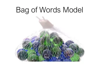
Bag-of-features – Origin: bag-of-words (text) • Orderless document representation: frequencies of words from a dictionary • Classification to determine document categories Bag-of-words Common 2 0 1 3 People 3 0 0 2 Sculpture 0 1 3 0 … … … … …

Bag-of-features for image classification SVM SVM Extract regions Compute Find clusters Compute distance Classification descriptors and frequencies matrix [Nowak,Jurie&Triggs,ECCV’06], [Zhang,Marszalek,Lazebnik&Schmid,IJCV’07]

Bag-of-features for image classification SVM SVM Extract regions Compute Find clusters Compute distance Classification descriptors and frequencies matrix Step 1 Step 3 Step 2 [Nowak,Jurie&Triggs,ECCV’06], [Zhang,Marszalek,Lazebnik&Schmid,IJCV’07]

Step 1: feature extraction • Scale-invariant image regions + SIFT (see lecture 2) – Affine invariant regions give “too” much invariance – Rotation invariance for many realistic collections “too” much invariance • Dense descriptors – Improve results in the context of categories (for most categories) – Interest points do not necessarily capture “all” features • Color-based descriptors • Shape-based descriptors

Dense features - Multi-scale dense grid: extraction of small overlapping patches at multiple scales -Computation of the SIFT descriptor for each grid cells -Exp.: Horizontal/vertical step size 6 pixel, scaling factor of 1.2 per level

Bag-of-features for image classification SVM SVM Extract regions Compute Find clusters Compute distance Classification descriptors and frequencies matrix Step 1 Step 3 Step 2

Step 2: Quantization …

Step 2:Quantization Clustering

Step 2: Quantization Visual vocabulary Clustering

Examples for visual words Airplanes Motorbikes Faces Wild Cats Leaves People Bikes

Step 2: Quantization • Cluster descriptors – K-means – Gaussian mixture model • Assign each visual word to a cluster • Assign each visual word to a cluster – Hard or soft assignment • Build frequency histogram

Gaussian mixture model (GMM) • Mixture of Gaussians: weighted sum of Gaussians where where

Hard or soft assignment • K-means � hard assignment – Assign to the closest cluster center – Count number of descriptors assigned to a center • Gaussian mixture model � soft assignment • Gaussian mixture model � soft assignment – Estimate distance to all centers – Sum over number of descriptors • Represent image by a frequency histogram

Image representation Image representation frequency fr ….. codewords • Each image is represented by a vector, typically 1000-4000 dimension, normalization with L1 norm • fine grained – represent model instances • coarse grained – represent object categories

Bag-of-features for image classification SVM SVM Extract regions Compute Find clusters Compute distance Classification descriptors and frequencies matrix Step 1 Step 3 Step 2

Step 3: Classification • Learn a decision rule (classifier) assigning bag-of- features representations of images to different classes Decision Zebra boundary Non-zebra Non-zebra

Training data Vectors are histograms, one from each training image positive negative Train classifier,e.g.SVM

Classification • Assign input vector to one of two or more classes • Any decision rule divides input space into decision regions separated by decision boundaries

Nearest Neighbor Classifier • Assign label of nearest training data point to each test data point ���������� ������ �������������������������������������� �������������������������������

k-Nearest Neighbors • For a new point, find the k closest points from training data • Labels of the k points “vote” to classify • Works well provided there is lots of data and the distance function is good k = 5 k = 5

Linear classifiers • Find linear function ( hyperplane ) to separate positive and negative examples ⋅ + ≥ positive : 0 x x w b i i ⋅ + < negative : 0 x x w b i i Which hyperplane is best?

Linear classifiers - margin x x 2 2 (color) (color) • Generalization is not good in this case: (roundness (roundness ) ) x x 1 1 x x 2 2 (color) (color) • Better if a margin is introduced: b/| | w (roundness (roundness ) ) x x 1 1