The story of the film so far... Experiments with integer outcomes - PowerPoint PPT Presentation
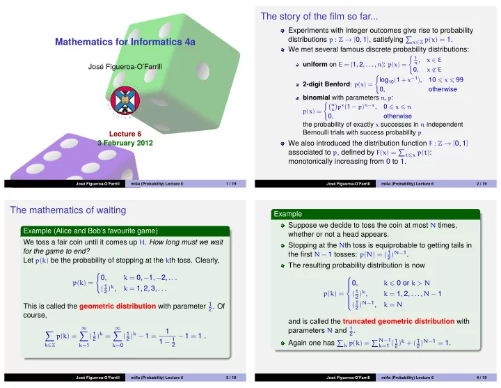
The story of the film so far... Experiments with integer outcomes give rise to probability distributions p : Z [ 0, 1 ] , satisfying x Z p ( x ) = 1. Mathematics for Informatics 4a We met several famous discrete probability
The story of the film so far... Experiments with integer outcomes give rise to probability distributions p : Z → [ 0, 1 ] , satisfying � x ∈ Z p ( x ) = 1. Mathematics for Informatics 4a We met several famous discrete probability distributions: � 1 n , x ∈ E uniform on E = { 1, 2, . . . , n } : p ( x ) = Jos´ e Figueroa-O’Farrill 0, x �∈ E � log 10 ( 1 + x − 1 ) , 10 � x � 99 2-digit Benford : p ( x ) = 0, otherwise binomial with parameters n , p : � � n p x ( 1 − p ) n − x , � 0 � x � n x p ( x ) = 0, otherwise the probability of exactly x successes in n independent Bernoulli trials with success probability p Lecture 6 3 February 2012 We also introduced the distribution function F : Z → [ 0, 1 ] associated to p , defined by F ( x ) = � t � x p ( t ) : monotonically increasing from 0 to 1. Jos´ e Figueroa-O’Farrill mi4a (Probability) Lecture 6 1 / 19 Jos´ e Figueroa-O’Farrill mi4a (Probability) Lecture 6 2 / 19 The mathematics of waiting Example Suppose we decide to toss the coin at most N times, Example (Alice and Bob’s favourite game) whether or not a head appears. We toss a fair coin until it comes up H . How long must we wait Stopping at the N th toss is equiprobable to getting tails in for the game to end? the first N − 1 tosses: p ( N ) = ( 1 2 ) N − 1 . Let p ( k ) be the probability of stopping at the k th toss. Clearly, The resulting probability distribution is now � 0, k = 0, − 1, − 2, . . . p ( k ) = 0, k � 0 or k > N ( 1 2 ) k , k = 1, 2, 3, . . . ( 1 2 ) k , p ( k ) = k = 1, 2, . . . , N − 1 ( 1 2 ) N − 1 , This is called the geometric distribution with parameter 1 k = N 2 . Of course, and is called the truncated geometric distribution with parameters N and 1 ∞ ∞ 2 . 1 � � � 2 ) k = 2 ) k − 1 = ( 1 ( 1 p ( k ) = − 1 = 1 . 1 − 1 Again one has � k p ( k ) = � N − 1 2 ) k + ( 1 2 ) N − 1 = 1. k = 1 ( 1 2 k ∈ Z k = 1 k = 0 Jos´ e Figueroa-O’Farrill mi4a (Probability) Lecture 6 3 / 19 Jos´ e Figueroa-O’Farrill mi4a (Probability) Lecture 6 4 / 19
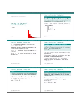
Geometric distribution Example (Dice instead of coins) Suppose that now Alice and Bob roll a fair die instead and the Definition game ends when one of them rolls a . What is the probability The geometric distribution with parameter p is given by p ( k ) that the game ends with the k th roll? . Then P ( S ) = 1 � Let S denote the event of rolling a 6 and hence ( 1 − p ) k − 1 p , k � 1 P ( S c ) = 5 p ( k ) = 6 . The game ends with the k th roll if the first k − 1 rolls 0, otherwise. do not show and the k th roll does. The probability of such a sequence of rolls is then The number p ( k ) is the probability that in independent Bernoulli � k − 1 1 � 5 6 , k � 1 trials with success probability p , the first success occurs at the 6 p ( k ) = k th trial. Notice that 0, otherwise. ∞ ∞ � � � ( 1 − p ) k − 1 p = p ( 1 − p ) ℓ p ( k ) = This is called the geometric distribution with parameter 1 6 . k ∈ Z k = 1 ℓ = 0 1 = p 1 − ( 1 − p ) = 1 . Jos´ e Figueroa-O’Farrill mi4a (Probability) Lecture 6 5 / 19 Jos´ e Figueroa-O’Farrill mi4a (Probability) Lecture 6 6 / 19 Negative binomial distribution Example (Weekly lottery) The binomial distribution answers the question: Let p be the probability that a given number d is drawn in any given week. After n successive draws, let p ( k ) be the Given n trials, what is the chance of k successes? probability that d last appeared k weeks ago. What is p ( k ) ? The number d appears with probability p and does not appear Suppose, instead, that we ask: with probability 1 − p . Then since d appeared k weeks ago and What is the chance we need n trials to obtain k successes? has not appeared since, we have � A Bernoulli trial is repeated until we attain k successes and let p ( 1 − p ) k , 0 � k � n − 1 p ( k ) = us call p k ( n ) the probability that the total number of trials is n . 0, otherwise If we need n trials, it is because there are k − 1 successes in the first n − 1 trials and the n th trial was a success. By Notice that independence, n − 1 � p ( k ) = 1 − ( 1 − p ) n , � n − 1 � � n − 1 � p k − 1 q n − k × p = p k q n − k p k ( n ) = k = 0 k − 1 k − 1 where ( 1 − p ) n is the probability that d does not appear in all n for n � k . This is the negative binomial distribution . weeks. Jos´ e Figueroa-O’Farrill mi4a (Probability) Lecture 6 7 / 19 Jos´ e Figueroa-O’Farrill mi4a (Probability) Lecture 6 8 / 19
Discrete random variables Examples We have seen how to assign a probability distribution to If Ω is finite then any function X : Ω → R is a discrete experiments with numerical (particularly, integer) random variable. outcomes. However not all interesting experiments are of In many practical situations, if Ω is a countable subset of R this type. (e.g., Ω = Z ) then the identity function X ( ω ) = ω is a Even if the outcomes are numerical, we may be interested discrete random variable. in some other numerical measure of the outcome; e.g., In the game of darts, Ω is uncountable since it contains all gamblers might be more interested in the monetary values the points in the dartboard on which the dart can land, but of their winnings/losses than in the actual number of times the score X : Ω → { 0, 1, . . . , 60 } is a discrete random that they win or lose. Such numerical measures are called variable. random variables . Notation Definition We will denote random variables by capital letters T , V , X , Y , Z , ... Let ( Ω , F , P ) be a probability space. A function X : Ω → R is a and their values by lowercase letters t , v , x , y , z , .... discrete random variable on ( Ω , F , P ) if it takes countably many values D = { x 1 , x 2 , . . . } ⊂ R , and 1 Please observe this convention very carefully!!! for every x i ∈ D , the set { ω ∈ Ω | X ( ω ) = x i } ∈ F . 2 Jos´ e Figueroa-O’Farrill mi4a (Probability) Lecture 6 9 / 19 Jos´ e Figueroa-O’Farrill mi4a (Probability) Lecture 6 10 / 19 Probability mass function Remarks Let X be a discrete random variable on a probability space In the case of Ω = Z and X being the identity function ( Ω , F , P ) taking integer values. (There is no loss of X ( ω ) = ω , f X ( x ) is what we called the probability generality in doing this, since any countable set can be distribution p ( x ) . labelled by integers.) Provided that we are only interested in X (and other By definition of a discrete random variable, the subset random variables we may build out of X ), we can A x = { ω ∈ Ω | X ( ω ) = x } of Ω is an event and therefore it has essentially forget about ( Ω , F , P ) and work with only the a well-defined probability P ( A x ) = P ( X = x ) . probability mass function f X . We often speak about “ a discrete random variable X with probability mass function This allows us to define a function f X by f X ( x ) = P ( X = x ) , called the probability mass function of X . f X ” without bothering to mention the probability space on which X is defined. Being a probability, 0 � f X ( x ) � 1 for all x ∈ R . The probability distributions we have been discussing can Since the A x for x ∈ Z are a countable partition of Ω , the play the rˆ ole of probability mass functions. countable additivity of P implies that One can talk about discrete random variables with uniform, � � � � � binomial, geometric, Benford,... probability mass functions. = P ( Ω ) = 1 . f X ( x ) = P ( A x ) = P A x x ∈ Z x ∈ Z x ∈ Z Jos´ e Figueroa-O’Farrill mi4a (Probability) Lecture 6 11 / 19 Jos´ e Figueroa-O’Farrill mi4a (Probability) Lecture 6 12 / 19
Recommend
More recommend
Explore More Topics
Stay informed with curated content and fresh updates.


