1 Hello Hi! My name is Ido, and we are going to talk about polar - PDF document
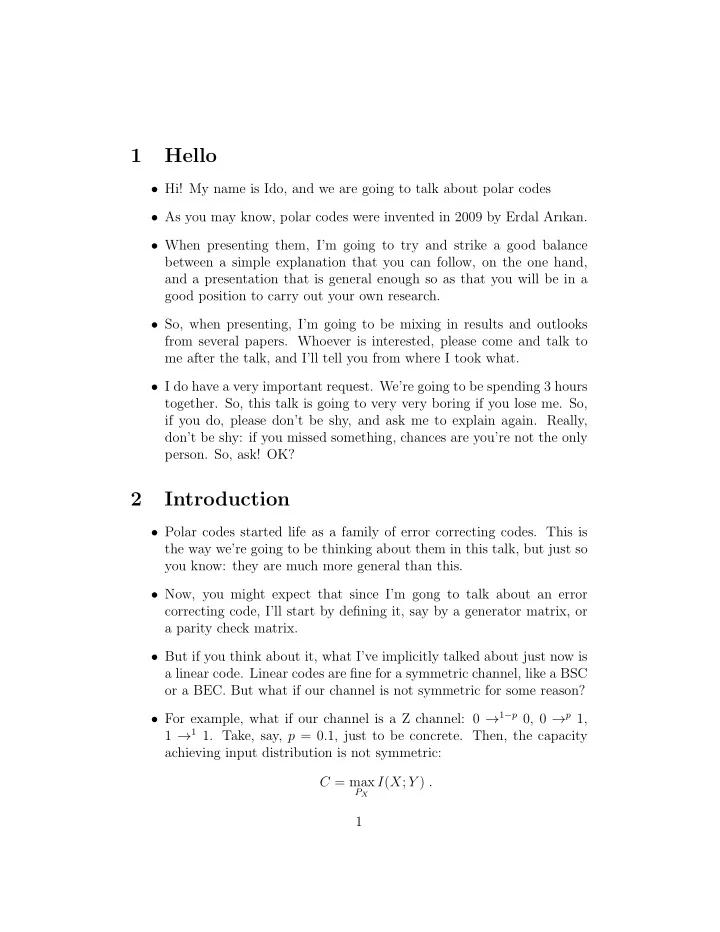
1 Hello Hi! My name is Ido, and we are going to talk about polar codes As you may know, polar codes were invented in 2009 by Erdal Arkan. When presenting them, Im going to try and strike a good balance between a simple explanation
1 Hello • Hi! My name is Ido, and we are going to talk about polar codes • As you may know, polar codes were invented in 2009 by Erdal Arıkan. • When presenting them, I’m going to try and strike a good balance between a simple explanation that you can follow, on the one hand, and a presentation that is general enough so as that you will be in a good position to carry out your own research. • So, when presenting, I’m going to be mixing in results and outlooks from several papers. Whoever is interested, please come and talk to me after the talk, and I’ll tell you from where I took what. • I do have a very important request. We’re going to be spending 3 hours together. So, this talk is going to very very boring if you lose me. So, if you do, please don’t be shy, and ask me to explain again. Really, don’t be shy: if you missed something, chances are you’re not the only person. So, ask! OK? 2 Introduction • Polar codes started life as a family of error correcting codes. This is the way we’re going to be thinking about them in this talk, but just so you know: they are much more general than this. • Now, you might expect that since I’m gong to talk about an error correcting code, I’ll start by defining it, say by a generator matrix, or a parity check matrix. • But if you think about it, what I’ve implicitly talked about just now is a linear code. Linear codes are fine for a symmetric channel, like a BSC or a BEC. But what if our channel is not symmetric for some reason? • For example, what if our channel is a Z channel: 0 → 1 − p 0, 0 → p 1, 1 → 1 1. Take, say, p = 0 . 1, just to be concrete. Then, the capacity achieving input distribution is not symmetric: C = max P X I ( X ; Y ) . 1
Since 1 is not as error prone, we’ll have P X (0) < 1 / 2 < P X (1). Not something a linear error correcting code handles well. • So, we’ll have to use something fancier than a linear code. • Also, you’ll need a bit of patience: we’ll get an error correcting scheme eventually, but we’ll start by defining concepts that will seem a bit abstract at first. You’ll have to trust me that everything will be useful in the end. • Let’s begin by defining the pair of random variables X and Y : X is a random variable having the input distribution we now fix, and Y is the random variable with a distribution corresponding to the output. So, think of X and Y as one input to the channel, and one corresponding output, respectively. • So, if X ∼ Ber( τ ) then, P X,Y ( X = x, Y = y ) = P X ( x ) · W ( y | x ), where W is the channel law and P X (1) = 1 − P X (0) = τ is our input distribution. I’ve written this in a different color since it is key concept that you should keep in mind, and I want to keep it on the board. • The previous step is important, so I should emphasize it: we are go- ing to build our polar code for a specific channel and a specific input distribution to the channel . You’d usually pick the capacity achieving input distribution to the channel, but you don’t have to. • The rate of our code is going to approach I ( X ; Y ) and the probability of error is going to approach 0. • Now, let’s define the pair of random vectors ( X N , Y N ) as N indepen- dent realizations of X and Y . That is, X N = ( X 1 , X 2 , . . . , X N ) is input to the channel, and Y N = ( Y 1 , Y 2 , . . . , Y N ) is the corresponding output. • OK, so ( X N , Y N ) is the first — for now abstract — concept that you need to remember. Let’s write it here, in a different color. 2
( X N , Y N ) • • Eventually, X N is going to be the input to the channel — the codeword, and Y N is going to be the channel output. However, we’re not there yet: for now, these are just mathematical definitions. • For simplicity, I’m going to assume a channel with binary input. So, X is going to be a binary random variable and X N is going to be a binary vector of length N . (write on board). • The second concept I need to tell you about is the Arıkan transform. It takes a vector x N of length N and transforms it into the vector u N = A ( x N ) . • The Arıkan transform is simple to define. However, I don’t want to burden you with the details just yet. Here is what I want you to know: – The Arıkan transform is one-to-one and onto. – Thus, there is also an inverse transform x N = A − 1 ( u N ). • Remember our pair of vectors, X N and Y N ? Let’s define U N = A ( X N ). • Our first result on polar codes is called slow polarization. Here it is Theorem 1: For every ǫ > 0, we have � �� i : H ( U i | Y N , U i − 1 ) < ǫ �� � lim = 1 − H ( X | Y ) N N →∞ and � �� i : H ( U i | Y N , U i − 1 ) > ǫ �� � lim = H ( X | Y ) . N N →∞ 3
• That’s quite a mouth-full. Let’s try and understand what I’ve just written. – Imagine that we are on the decoder side. So, we get to see Y N . So, having, Y N on the conditioning side makes sense. – You usually think of the decoder as trying to figure out the code- word, this is going to be X N , from the received word, which is going to be Y N . – However, since the polar transform is invertible, we might just as well try to figure out U N for Y N . That is, we will guess ˆ U N , and X N = A − 1 ( ˆ from this guess that the codeword was ˆ U N ) – Suppose that our decoder is trying to figure out U i , and, for some reason that I will justify later, someone tells us the what U i − 1 was. – Then, for N large enough, for a fraction of 1 − H ( X | Y ) indices, this is going to be “easy”. That is, if ǫ is small and H ( U i | U i − 1 , Y N ) < ǫ , then the entropy of U i given the above is very small: the decoder has a very good chance of guessing it correctly. – Conversely, if ǫ is very small and H ( U i | U i − 1 , Y N ) > 1 − ǫ , then the decoder has an almost fifty-fifty chance of guessing U i correctly, given that it has seen Y N and has been told U i − 1 . So, in this case, we don’t want to risk the decoder making the wrong guess, and we will “help” it. How, we’ll see. . . • In order to show that the probability of misdecoding goes down to 0 with N , we will need a stronger theorem. Theorem 2: For every 0 < β < 1 / 2, we have � � i : H ( U i | Y N , U i − 1 ) < 2 − N β �� � � � � lim = 1 − H ( X | Y ) N N →∞ and � � i : H ( U i | Y N , U i − 1 ) > 1 − 2 − N β �� � � � � lim = H ( X | Y ) . N N →∞ 4
• The above already gives us a capacity achieving coding scheme for any symmetric channel. Namely, for any channel for which the capacity achieving input distribution is P X (0) = P X (1) = 1 / 2. • Assume that W is such a channel, and take P X (0) = P X (1) = 1 / 2. – So, all realizations x N ∈ { 0 , 1 } N of X N are equally likely. – That is, for all x N ∈ { 0 , 1 } N , we have P ( X N = x N ) = 1 / 2 N . – That means that for all u N ∈ { 0 , 1 } N , we have P ( U N = u N ) = 1 / 2 N . – Fix β < 1 / 2. Say, β = 0 . 4. Take � i : P err ( U i | Y N , U i − 1 ) ≥ 2 − N β � F = , F c = � i : P err ( U i | Y N , U i − 1 ) < 2 − N β � |F c | = k , – Just to be clear, for a binary random variable A , � P err ( A | B ) = P ( A = a, B = b ) ( a,b ) � · [ P ( A = a | B = b ) < P ( A = 1 − a | B = b )] + 1 � 2[ P ( A = a | B = b ) = P ( A = 1 − a | B = b )] – That is, the probability of misdecoding A by an optimal (ML) decoder seeing B . – Theorem 2 continues to hold if H ( . . . ) is replaced by 2P err ( . . . ). – The first set is called “Frozen”, since it will be frozen to some known value before transmission. That analogy won’t be great when we move to a non-systematic setting, so don’t get too at- tached to it. – We are going to transmit k information bits. – The rate R = k/N will approach 1 − H ( X | Y ), by Theorem 1 (with 2P err in place of H , and fiddling with β ). 5
– In our case 1 − H ( X | Y ) = I ( X ; Y ), the capacity. – Let’s “build” U N using our information bits, and then make sure that our U N indeed has the right distribution. – We will put k information bits into the U i for which P err ( U i | Y N , U i − 1 ) < 2 − N β . – Assumption: the information bits are i.i.d. Ber(1 / 2). This is a fair assumption: otherwise, we have not fully compressed the source. – Anyway, we can always make this assumption valid by XORing our input bits with an i.i.d. Ber(1 / 2) vector, and then undoing this operation in the end. – In the remaining N − k entries, U i will contain i.i.d. Ber(1 / 2) bits, chosen in advance and known to both the encoder and the decoder. – The resulting vector U N has the correct probability distribution: all values are equally likely. – Since we’ve built U N , we’ve also built X N = A − 1 ( U N ). That is what the encoder transmits over the channel. – Now, let’s talk about decoding. – Let u N , x N , y N denote the realizations of U N , X N , Y N . – The decoder sees y N , and has to guess u N . Denote that guess by u N . ˆ – We will decode sequentially, first ˆ u 1 , then guess ˆ u 2 , . . . , and finally u N . ˆ – At stage i , when decoding ˆ u i , there are two possibilities: ∗ ˆ u i does not contain one of the k information bits. ∗ ˆ u i contains one of the k information bits. – The first case is easy: everybody, including the decoder, knows the value of u i . So, simply set ˆ u i = u i . – In the second case, we set 6
Recommend
More recommend
Explore More Topics
Stay informed with curated content and fresh updates.

