BBM406 Fundamentals of Machine Learning Lecture 4: Linear - PowerPoint PPT Presentation

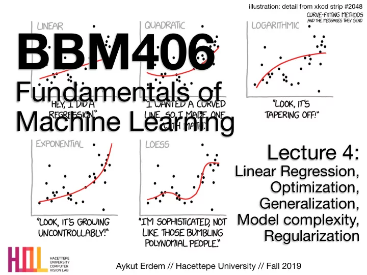
illustration: detail from xkcd strip #2048 BBM406 Fundamentals of 
 Machine Learning Lecture 4: Linear Regression, Optimization, Generalization, Model complexity, Regularization Aykut Erdem // Hacettepe University // Fall 2019

𝑦 1 , 𝑧 1 , … , 𝑦 𝑜 , 𝑧 𝑜 • 𝑦 𝑗 ∈ 𝑌 – 𝑧 𝑗 ∈ ℜ – • 𝐿 ∶ 𝑌 × 𝑌 → ℜ – – • Recall from last time… Kernel Regression – x’ ′ 𝐿 𝑦 𝑗 , 𝑦 – Here, this is Here, this is the closest the closest Here, this is the closest Here, this is the closest y x 1-NN for Regression Weighted K-NN for Regression ! 1 /p n X | x i − y i | p D = w i = exp(-d(x i , query) 2 / σ 2 ) i =1 Distance metrics Kernel width 2

Linear Regression 3


 
 Simple 1-D Regression • Circles are data points (i.e., training examples) that are given to us • The data points are uniform in x , but may be displaced in y 
 t ( x ) = f ( x ) + ε 
 with ε some noise slide by Sanja Fidler • In green is the “true” curve that we don’t know 
 • Goal: We want to fit a curve to these points 4

Simple 1-D Regression • Key Questions: − How do we parametrize the model (the curve)? − What loss (objective) function should we use to judge fit? − How do we optimize fit to unseen test data slide by Sanja Fidler ( generalization )? 
 5

Example: Boston House Prizes • Estimate median house price in a neighborhood based on neighborhood statistics • Look at first (of 13) attributes: per capita crime rate slide by Sanja Fidler • Use this to predict house prices in other neighborhoods Is this a good input (attribute) to predict house prices? • https://archive.ics.uci.edu/ml/datasets/Housing 6


 Represent the data • Data described as pairs D = {( x (1) , t (1) ), ( x (2) , t (2) ),..., ( x ( N ) , t ( N ) )} − x is the input feature (per capita crime rate) − t is the target output (median house price) − ( i ) simply indicates the training examples (we have N in this case) • Here t is continuous, so this is a regression problem • Model outputs y, an estimate of t 
 y ( x ) = w 0 + w 1 x • What type of model did we choose? • Divide the dataset into training and testing examples slide by Sanja Fidler − Use the training examples to construct hypothesis, or function approximator, that maps x to predicted y − Evaluate hypothesis on test set 7

Noise • A simple model typically does not exactly fit the data — lack of fit can be considered noise 
 • Sources of noise: − Imprecision in data attributes (input noise, e.g. noise in per-capita crime) − Errors in data targets (mislabeling, e.g. noise in house prices) − Additional attributes not taken into account by data attributes, a ff ect target values (latent variables). In the example, what else could a ff ect house prices? − Model may be too simple to account for data targets slide by Sanja Fidler 8

Least-Squares Regression y ( x ) = function( x, w ) slide by Sanja Fidler 9


 
 Least-Squares Regression • Define a model 
 Linear: y ( x ) = function( x, w ) • Standard loss/cost/objective function measures the squared error between y and the true value t 
 slide by Sanja Fidler • For a particular hypothesis ( y ( x ) defined by a choice of w , drawn in red), what does the loss represent geometrically? 10


 
 Least-Squares Regression • Define a model 
 Linear: y ( x ) = w 0 + w 1 x • Standard loss/cost/objective function measures the squared error between y and the true value t 
 slide by Sanja Fidler • For a particular hypothesis ( y ( x ) defined by a choice of w , drawn in red), what does the loss represent geometrically? 11


 
 Least-Squares Regression • Define a model 
 Linear: y ( x ) = w 0 + w 1 x • Standard loss/cost/objective function measures the squared error between y and the true value t 
 N i 2 h X t ( n ) − y ( x ( n ) ) ` ( w ) = slide by Sanja Fidler n =1 • For a particular hypothesis ( y ( x ) defined by a choice of w , drawn in red), what does the loss represent geometrically? 12


 
 Least-Squares Regression • Define a model 
 Linear: y ( x ) = w 0 + w 1 x • Standard loss/cost/objective function measures the squared error between y and the true value t 
 N i 2 h X t ( n ) − ( w 0 + w 1 x ( n ) ) Linear model: ` ( w ) = slide by Sanja Fidler n =1 • For a particular hypothesis ( y ( x ) defined by a choice of w , drawn in red), what does the loss represent geometrically? 13


 
 Least-Squares Regression • Define a model 
 Linear: y ( x ) = w 0 + w 1 x • Standard loss/cost/objective function measures the squared error between y and the true value t 
 N i 2 h X t ( n ) − ( w 0 + w 1 x ( n ) ) Linear model: ` ( w ) = slide by Sanja Fidler n =1 • For a particular hypothesis ( y ( x ) defined by a choice of w , drawn in red), what does the loss represent geometrically? 14


 
 Least-Squares Regression • Define a model 
 Linear: y ( x ) = w 0 + w 1 x • Standard loss/cost/objective function measures the squared error between y and the true value t 
 N i 2 h X t ( n ) − ( w 0 + w 1 x ( n ) ) Linear model: ` ( w ) = slide by Sanja Fidler n =1 • The loss for the red hypothesis is the sum of the squared vertical errors (squared lengths of green vertical lines) 15


 
 Least-Squares Regression • Define a model 
 Linear: y ( x ) = w 0 + w 1 x • Standard loss/cost/objective function measures the squared error between y and the true value t 
 N i 2 h X t ( n ) − ( w 0 + w 1 x ( n ) ) Linear model: ` ( w ) = slide by Sanja Fidler n =1 • How do we obtain weights ? 
 w = ( w 0 , w 1 ) 16


 
 Least-Squares Regression • Define a model 
 Linear: y ( x ) = w 0 + w 1 x • Standard loss/cost/objective function measures the squared error between y and the true value t 
 N i 2 h X t ( n ) − ( w 0 + w 1 x ( n ) ) Linear model: ` ( w ) = slide by Sanja Fidler n =1 • How do we obtain weights ? Find w that minimizes 
 w = ( w 0 , w 1 ) loss ` ( w ) 17

Optimizing the Objective • One straightforward method: gradient descent − initialize w (e.g., randomly) − repeatedly update w based on the gradient 
 w ← w − � @` @ w • λ is the learning rate • For a single training case, this gives the LMS update rule: ⇣ ⌘ t ( n ) − y ( x ( n ) ) x ( n ) w ← w + 2 λ { error slide by Sanja Fidler • Note: As error approaches zero, so does the update 
 ( w stops changing) 18

19 Optimizing the Objective slide by Fei-Fei Li & Andrej Karpathy & Justin Johnson

20 Optimizing the Objective slide by Fei-Fei Li & Andrej Karpathy & Justin Johnson

E ff ect of learning rate λ ` ( w ) ` ( w ) w 0 w 0 • Large λ => Fast convergence but larger residual error 
 Also possible oscillations slide by Erik Sudderth • Small λ => Slow convergence but small residual error 21

Optimizing Across Training Set • Two ways to generalize this for all examples in training set: 1. Batch updates: sum or average updates across every example n, then change the parameter values ⇣ ⌘ t ( n ) − y ( x ( n ) ) x ( n ) w ← w + 2 λ 2. Stochastic/online updates: update the parameters for each training case in turn, according to its own gradients Algorithm 1 Stochastic gradient descent 1: Randomly shu ffl e examples in the training set 2: for i = 1 to N do Update: 3: slide by Sanja Fidler w ← w + 2 λ ( t ( i ) − y ( x ( i ) )) x ( i ) (update for a linear model) 4: end for 22

Optimizing Across Training Set • Two ways to generalize this for all examples in training set: 1. Batch updates: sum or average updates across every example n, then change the parameter values ⇣ ⌘ t ( n ) − y ( x ( n ) ) x ( n ) w ← w + 2 λ 2. Stochastic/online updates: update the parameters for each training case in turn, according to its own gradients • Underlying assumption: sample is independent and identically distributed (i.i.d.) slide by Sanja Fidler 23

Analytical Solution • For some objectives we can also find the optimal solution analytically • This is the case for linear least-squares regression • How? slide by Sanja Fidler 24

Vectorization • Consider our model: y ( x ) = w 0 + w 1 x • Let  w 0 � x T = [1 x ] w = w 1 • Can write the model in vectorized form as y ( x ) = w T x 25


 Vectorization • Consider our model with N instances: 
 R N × 1 t (1) , t (2) , . . . , t ( N ) i T h t = T 1 , x (1) 2 3 R N × 2 1 , x (2) 6 7 X = 6 7 . . . 4 5 1 , x ( N ) R 2 × 1  w 0 � w = w 1 • Then: 
 N w T x ( n ) − t ( n ) i 2 h X ` ( w ) = slide by Sanja Fidler n =1 = ( Xw − t ) T ( Xw − t ) { { R 1 × N R N × 1 26