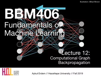
BBM406 Fundamentals of Machine Learning Lecture 17: Kernel Trick - PowerPoint PPT Presentation

Photo by Arthur Gretton, CMU Machine Learning Protestors at G20 BBM406 Fundamentals of 
 Machine Learning Lecture 17: Kernel Trick for SVMs Risk and Loss Support Vector Regression Aykut Erdem // Hacettepe University // Fall 2019

Administrative Deadlines are much closer than they appear • Project progress reports are 
 on syllabus due soon! 
 Due: December 22, 2019 (11:59pm) Each group should submit a project progress report by December 22, 2018. The report should be 3-4 pages and should describe the following points as clearly as possible: • Problem to be addressed. Give a short description of the problem that you will explore. Explain why you find it interesting. • Related work. Briefly review the major works related to your research topic. • Methodology to be employed. Describe the neural architecture that is expected to form the basis of the project. State whether you will extend an existing method or you are going to devise your own approach. • Experimental evaluation. Briefly explain how you will evaluate your results. State which dataset(s) you will employ in your evaluation. Provide your preliminary results (if any). 2

Last time… Soft-margin Classifier h w, x i + b � 1 h w, x i + b  � 1 minimum error separator is impossible Theorem (Minsky & Papert) 
 slide by Alex Smola Finding the minimum error separating hyperplane is NP hard

Last time… Adding Slack Variables ξ i ≥ 0 h w, x i + b � 1 � ξ h w, x i + b  � 1 + ξ minimize amount of slack slide by Alex Smola Convex optimization problem

Last time… Adding Slack Variables • for point is between the margin and correctly 0 < ξ ≤ 1 classified • for point is misclassified ξ i ≥ 0 h w, x i + b � 1 � ξ h w, x i + b  � 1 + ξ adopted from Andrew Zisserman minimize amount of slack Convex optimization problem


 
 
 Last time… Adding Slack Variables • Hard margin problem 1 2 k w k 2 subject to y i [ h w, x i i + b ] � 1 minimize w,b • With slack variables 
 1 2 k w k 2 + C X minimize ξ i w,b i subject to y i [ h w, x i i + b ] � 1 � ξ i and ξ i � 0 Problem is always feasible. Proof: 
 (also yields upper bound) w = 0 and b = 0 and ξ i = 1 slide by Alex Smola


 
 
 Soft-margin classifier • Optimization problem: 
 1 2 k w k 2 + C X minimize ξ i w,b i subject to y i [ h w, x i i + b ] � 1 � ξ i and ξ i � 0 C is a regularization parameter: • small C allows constraints to be easily ignored 
 → large margin • large C makes constraints hard to ignore 
 adopted from Andrew Zisserman → narrow margin • C = ∞ enforces all constraints: hard margin

Last time… Multi-class SVM • Simultaneously-learn-3-sets-- w + of-weights:-- w - • How-do-we-guarantee-the-- correct-labels?-- w o • Need-new-constraints!-- The-“score”-of-the-correct-- class-must-be-be?er-than- the-“score”-of-wrong-classes:-- slide by Eric Xing 8

Last time… Multi-class SVM • As#for#the#SVM,#we#introduce#slack#variables#and#maximize#margin:## To predict, we use: Now#can#we#learn#it?### ?  slide by Eric Xing 9

Last time… Kernels • Original data • Data in feature space (implicit) • Solve in feature space using kernels slide by Alex Smola 10

Last time… Quadratic Features Quadratic Features in Quadratic Features in R 2 p ⇣ ⌘ x 2 2 x 1 x 2 , x 2 Φ ( x ) := 1 , 2 Dot Product Dot Product p p D⇣ ⌘ ⇣ 2 ⌘E 2 , h Φ ( x ) , Φ ( x 0 ) i = x 0 2 x 0 1 x 0 2 , x 0 x 2 2 x 1 x 2 , x 2 1 , , 2 1 2 = h x, x 0 i 2 . Insight Insight Trick works for any polynomials of order via Trick works for any polynomials of order d via h x, x 0 i d . slide by Alex Smola 11

Computational E ffi ciency Problem Extracting features can sometimes be very costly. Example: second order features in 1000 dimensions. This leads to 5005 numbers. For higher order polyno- 5 · 10 5 mial features much worse. Solution Solution Don’t compute the features, try to compute dot products implicitly. For some features this works . . . Definition Definition A kernel function k : X ⇥ X ! R is a symmetric function in its arguments for which the following property holds k ( x, x 0 ) = h Φ ( x ) , Φ ( x 0 ) i for some feature map Φ . slide by Alex Smola If k ( x, x 0 ) is much cheaper to compute than Φ ( x ) . . . 12

Last time.. Example kernels Examples of kernels k ( x, x 0 ) h x, x 0 i Linear exp ( � λ k x � x 0 k ) Laplacian RBF � λ k x � x 0 k 2 � � Gaussian RBF exp ( h x, x 0 i + c i ) d , c � 0 , d 2 N Polynomial B 2 n +1 ( x � x 0 ) B-Spline E c [ p ( x | c ) p ( x 0 | c )] Cond. Expectation Simple trick for checking Mercer’s condition Compute the Fourier transform of the kernel and check that it is nonnegative. slide by Alex Smola 13

Today • The Kernel Trick for SVMs • Risk and Loss • Support Vector Regression 14

The Kernel Trick for SVMs slide by Alex Smola


 
 The Kernel Trick for SVMs • Linear soft margin problem 1 2 k w k 2 + C X minimize ξ i w,b i subject to y i [ h w, x i i + b ] � 1 � ξ i and ξ i � 0 • Dual problem 
 � 1 X X maximize α i α j y i y j h x i , x j i + α i 2 α i,j i X subject to α i y i = 0 and α i 2 [0 , C ] i • Support vector expansion slide by Alex Smola X f ( x ) = α i y i h x i , x i + b i


 
 The Kernel Trick for SVMs • Linear soft margin problem 1 2 k w k 2 + C X minimize ξ i w,b i subject to y i [ h w, φ ( x i ) i + b ] � 1 � ξ i and ξ i � 0 • Dual problem 
 − 1 X X maximize α i α j y i y j k ( x i , x j ) + α i 2 α i,j i X subject to α i y i = 0 and α i ∈ [0 , C ] i • Support vector expansion slide by Alex Smola X f ( x ) = α i y i k ( x i , x ) + b i

C=1 slide by Alex Smola

C=1 y = 1 support 
 vectors y = -1 y=0 support 
 vectors slide by Alex Smola

C=2 slide by Alex Smola

C=5 slide by Alex Smola

C=10 slide by Alex Smola

C=20 slide by Alex Smola

C=50 slide by Alex Smola

C=100 slide by Alex Smola

C=1 slide by Alex Smola

C=2 slide by Alex Smola

C=5 slide by Alex Smola

C=10 slide by Alex Smola

C=20 slide by Alex Smola

C=50 slide by Alex Smola

C=100 slide by Alex Smola

C=1 slide by Alex Smola

C=2 slide by Alex Smola

C=5 slide by Alex Smola

C=10 slide by Alex Smola

C=20 slide by Alex Smola

C=50 slide by Alex Smola

C=100 slide by Alex Smola

C=1 slide by Alex Smola

C=2 slide by Alex Smola

C=5 slide by Alex Smola

C=10 slide by Alex Smola

C=20 slide by Alex Smola

C=50 slide by Alex Smola

C=100 slide by Alex Smola

And now with a narrower kernel slide by Alex Smola

slide by Alex Smola

slide by Alex Smola

slide by Alex Smola

slide by Alex Smola

And now with a very wide kernel slide by Alex Smola

slide by Alex Smola

Nonlinear Separation • Increasing C allows for more nonlinearities • Decreases number of errors • SV boundary need not be contiguous slide by Alex Smola • Kernel width adjusts function class

Overfitting? • Huge feature space with kernels: should we worry about overfitting? 
 • SVM objective seeks a solution with large margin - Theory says that large margin leads to good generalization (we will see this in a couple of lectures) 
 • But everything overfits sometimes!!! 
 • Can control by: - Setting C - Choosing a better Kernel - Varying parameters of the Kernel (width of Gaussian, slide by Alex Smola etc.) 55

56 Risk and Loss slide by Alex Smola


 
 
 
 
 Loss function point of view • Constrained quadratic program 
 1 2 k w k 2 + C X minimize ξ i w,b i subject to y i [ h w, x i i + b ] � 1 � ξ i and ξ i � 0 • Risk minimization setting 
 1 2 k w k 2 + C X minimize max [0 , 1 � y i [ h w, x i i + b ]] w,b i empirical risk Follows from finding minimal slack variable slide by Alex Smola for given ( w,b ) pair.

Soft margin as proxy for binary • Soft margin loss max(0 , 1 − yf ( x )) • Binary loss { yf ( x ) < 0 } convex upper bound binary loss function margin slide by Alex Smola

More loss functions h 1 + e − f ( x ) i • Logistic log • Huberized loss  0 if f ( x ) > 1   2 (1 − f ( x )) 2 1 if f ( x ) ∈ [0 , 1] 1  2 − f ( x ) if f ( x ) < 0  • Soft margin (asymptotically) linear max(0 , 1 − f ( x )) (asymptotically) 0 slide by Alex Smola


 
 
 Risk minimization view • Find function f minimizing classification error R [ f ] := E x,y ∼ p ( x,y ) [ { yf ( x ) > 0 } ] • Compute empirical average 
 m R emp [ f ] := 1 X { y i f ( x i ) > 0 } m i =1 − Minimization is nonconvex − Overfitting as we minimize empirical error • Compute convex upper bound on the loss • Add regularization for capacity control 
 regularization m R reg [ f ] := 1 X max(0 , 1 − y i f ( x i )) + λ Ω [ f ] slide by Alex Smola m i =1 how to control ƛ

Support Vector 
 Regression 61