The Paradox of Overfitting Volker Nannen February 1, 2003 - PowerPoint PPT Presentation

The Paradox of Overfitting Volker Nannen February 1, 2003 Artificial Intelligence Rijksuniversiteit Groningen

Contents 1. MDL – theory 2. Experimental Verification 3. Results

MDL – theory

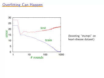
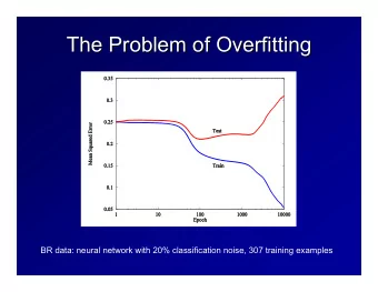
1.1 the problem The paradox of overfitting: Complex models contain more information on the training data but less information on future data. - 2 -

1.2 model selection Machine learning uses models to describe reality. - 3 -

1.2 model selection Models can be • statistical distributions • polynomials • Markov chains • neural networks • decision trees • etc. - 4 -

1.2 model selection This work uses polynomial models. m k = p k ( x ) = a 0 + · · · + a k x k (1) Polynomials are • well understood • used throughout mathematics • suffer badly from overfitting - 5 -

1.3 mean squared error The mean squared error of a model m on a sample s = { ( x 1 , y 1 ) . . . ( x n , y n ) } (2) of size n is n f = 1 � � 2 σ 2 � m ( x i ) − y i (3) n i =0 - 6 -

1.3 mean squared error The error on the training sample is called training error. The error on future samples is called generalization error. We want to minimize the generalization error. - 7 -

1.4 an example of overfitting An example of overfitting: regression in the two-dimensional plane - 8 -

1.4 an example of overfitting Continuous signal + noise, 300 point sample. - 9 -

1.4 an example of overfitting 6 degree polynomial, σ 2 = 13 . 8 - 10 -

1.4 an example of overfitting 17 degree polynomial, σ 2 = 5 . 8 - 11 -

1.4 an example of overfitting 43 degree polynomial, σ 2 = 1 . 5 - 12 -

1.4 an example of overfitting 100 degree polynomial, σ 2 = 0 . 6 - 13 -

1.4 an example of overfitting 3,000 point test sample. σ 2 t = 10 12 - 14 -

1.4 an example of overfitting Generalization error on this 3,000 point test sample. σ 2 = 16 , σ 2 = 8 . 6 , 6 degree: 17 degree: σ 2 = 2 . 7 , σ 2 = 10 12 . 43 degree: 100 degree: - 15 -

1.5 Minimum Description Length Rissanens hypothesis: Minimum Description Length prevents overfitting. - 16 -

1.5 Minimum Description Length MDL minimizes the code length � � min l ( s | m ) + l ( m ) (4) m This is a two-part code: l ( m ) is the code length of the model and l ( s | m ) is the code length of the data given the model. - 17 -

1.5 Minimum Description Length We only look at the least square model per degree � � min n log ˆ σ m k + l ( m ) (5) k Rissanen’s original estimation: σ m k + k log √ n � � min n log ˆ (6) k This is too weak. - 18 -

1.5 Minimum Description Length Mixture MDL is a modern version of MDL. � � � min − log p ( M k = m k ) p ( s | m k ) d m k (7) k m k ∈ M k p ( M k = m k ) is a prior distribution over models in M k . Barron & Liang provide a simple algorithm based on the uniform prior (2002). - 19 -

Experimental Verification

2.1 the problem Problems with experiments on model selection: • shortage of appropriate data • inefficient setup of experiments • insufficient visualization • few tangible results - 21 -

2.2 the solution Solution: The Statistical Data Viewer an advanced tool for statistical experiments. - 22 -

2.3 A simple experiment A simple experiment: the sinus wave - 23 -

2.3 A simple experiment A new project - 24 -

2.3 A simple experiment A new process and sample - 25 -

2.3 A simple experiment Selecting a method for a model - 26 -

2.3 A simple experiment Analyzing the generalization error - 27 -

2.3 A simple experiment Analysis, cross validation, mixture MDL and Rissanen’s MDL. Optimum at 0 degrees. - 28 -

2.3 A simple experiment 150 point sample. Optimum at 17 degrees. - 29 -

2.3 A simple experiment 300 point sample. Optimum at 18 degrees. - 30 -

Results

3.1 achievements Achievements: • generic problem space (files, broad selection of online signals, drawing by hand) • graphical object oriented setup of experiments (no scripting) • graphics integrated into the control structure • simple programming interfaces - 32 -

3.2 Conclusion Conclusion for all experiments: • Rissanens original version usually overfits. • Mixture MDL can prevent overfitting. • smoothing is important for model selection. • Mixture MDL cannot deal with non-uniform support. (but cross validation can do it!) • Mixture MDL can deal with different types of noise. (i.i.d. assumption can be relaxed!) • The structure of a prediction graph contains valuable information by itself and MDL can reproduce it. - 33 -

3.3 further research Further research: • The structure of the generalization error • Other types of data • Other types of models • Improved interfaces - 34 -

volker.nannen.com/mdl