Markov Decision Processes Philipp Koehn presented by Shuoyang Ding - PowerPoint PPT Presentation
Markov Decision Processes Philipp Koehn presented by Shuoyang Ding 11 April 2017 Philipp Koehn Artificial Intelligence: Markov Decision Processes 11 April 2017 Outline 1 Hidden Markov models Inference: filtering, smoothing, best
Markov Decision Processes Philipp Koehn presented by Shuoyang Ding 11 April 2017 Philipp Koehn Artificial Intelligence: Markov Decision Processes 11 April 2017
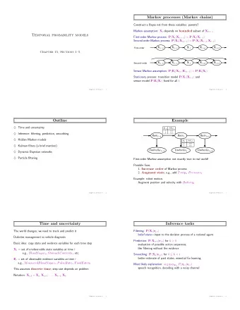
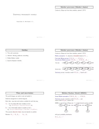
Outline 1 ● Hidden Markov models ● Inference: filtering, smoothing, best sequence ● Kalman filters (a brief mention) ● Dynamic Bayesian networks ● Speech recognition Philipp Koehn Artificial Intelligence: Markov Decision Processes 11 April 2017
Time and Uncertainty 2 ● The world changes; we need to track and predict it ● Diabetes management vs vehicle diagnosis ● Basic idea: sequence of state and evidence variables ● X t = set of unobservable state variables at time t e.g., BloodSugar t , StomachContents t , etc. ● E t = set of observable evidence variables at time t e.g., MeasuredBloodSugar t , PulseRate t , FoodEaten t ● This assumes discrete time ; step size depends on problem ● Notation: X a ∶ b = X a , X a + 1 ,..., X b − 1 , X b Philipp Koehn Artificial Intelligence: Markov Decision Processes 11 April 2017
Markov Processes (Markov Chains) 3 ● Construct a Bayes net from these variables: parents? ● Markov assumption: X t depends on bounded subset of X 0 ∶ t − 1 ● First-order Markov process: P ( X t ∣ X 0 ∶ t − 1 ) = P ( X t ∣ X t − 1 ) Second-order Markov process: P ( X t ∣ X 0 ∶ t − 1 ) = P ( X t ∣ X t − 2 , X t − 1 ) ● Sensor Markov assumption: P ( E t ∣ X 0 ∶ t , E 0 ∶ t − 1 ) = P ( E t ∣ X t ) ● Stationary process: transition model P ( X t ∣ X t − 1 ) and sensor model P ( E t ∣ X t ) fixed for all t Philipp Koehn Artificial Intelligence: Markov Decision Processes 11 April 2017
Example 4 ● First-order Markov assumption not exactly true in real world! ● Possible fixes: 1. Increase order of Markov process 2. Augment state , e.g., add Temp t , Pressure t Philipp Koehn Artificial Intelligence: Markov Decision Processes 11 April 2017
5 inference Philipp Koehn Artificial Intelligence: Markov Decision Processes 11 April 2017
Inference Tasks 6 ● Filtering: P ( X t ∣ e 1 ∶ t ) belief state—input to the decision process of a rational agent ● Smoothing: P ( X k ∣ e 1 ∶ t ) for 0 ≤ k < t better estimate of past states, essential for learning ● Most likely explanation: arg max x 1 ∶ t P ( x 1 ∶ t ∣ e 1 ∶ t ) speech recognition, decoding with a noisy channel Philipp Koehn Artificial Intelligence: Markov Decision Processes 11 April 2017
Filtering 7 ● Aim: devise a recursive state estimation algorithm P ( X t + 1 ∣ e 1 ∶ t + 1 ) = P ( X t + 1 ∣ e 1 ∶ t , e t + 1 ) = α P ( e t + 1 ∣ X t + 1 , e 1 ∶ t ) P ( X t + 1 ∣ e 1 ∶ t ) (Bayes rule) = α P ( e t + 1 ∣ X t + 1 ) P ( X t + 1 ∣ e 1 ∶ t ) (Sensor Markov assumption) = α P ( e t + 1 ∣ X t + 1 )∑ P ( X t + 1 ∣ x t , e 1 ∶ t ) P ( x t ∣ e 1 ∶ t ) (multiplying out) x t = α P ( e t + 1 ∣ X t + 1 )∑ P ( X t + 1 ∣ x t ) P ( x t ∣ e 1 ∶ t ) (first order Markov model) x t ● Summary: P ( X t + 1 ∣ e 1 ∶ t + 1 ) = α P ( e t + 1 ∣ X t + 1 ) P ( X t + 1 ∣ x t ) P ( x t ∣ e 1 ∶ t ) ∑ �ÜÜÜÜÜÜÜÜÜÜÜÜÜÜÜÜÜÜÜÜÜÜÜÜÜÜÜÜÜ�ÜÜÜÜÜÜÜÜÜÜÜÜÜÜÜÜÜÜÜÜÜÜÜÜÜÜÜÜÜ� �ÜÜÜÜÜÜÜÜÜÜÜÜÜÜÜÜÜÜÜÜÜ�ÜÜÜÜÜÜÜÜÜÜÜÜÜÜÜÜÜÜÜÜÜÜ� �ÜÜÜÜÜÜÜÜÜÜÜÜÜÜÜÜÜÜÜ�ÜÜÜÜÜÜÜÜÜÜÜÜÜÜÜÜÜÜÜ� x t emission transition recursive call ● f 1 ∶ t + 1 = F ORWARD ( f 1 ∶ t , e t + 1 ) where f 1 ∶ t = P ( X t ∣ e 1 ∶ t ) Time and space constant (independent of t ) Philipp Koehn Artificial Intelligence: Markov Decision Processes 11 April 2017
Filtering Example 8 transition transition emission emission Philipp Koehn Artificial Intelligence: Markov Decision Processes 11 April 2017
Smoothing 9 ● If full sequence is known ⇒ what is the state probability P ( X k ∣ e 1 ∶ t ) including future evidence? ● Smoothing: sum over all paths Philipp Koehn Artificial Intelligence: Markov Decision Processes 11 April 2017
Smoothing 10 ● Divide evidence e 1 ∶ t into e 1 ∶ k , e k + 1 ∶ t : P ( X k ∣ e 1 ∶ t ) = P ( X k ∣ e 1 ∶ k , e k + 1 ∶ t ) = α P ( X k ∣ e 1 ∶ k ) P ( e k + 1 ∶ t ∣ X k , e 1 ∶ k ) = α P ( X k ∣ e 1 ∶ k ) P ( e k + 1 ∶ t ∣ X k ) = α f 1 ∶ k b k + 1 ∶ t ● Backward message b k + 1 ∶ t computed by a backwards recursion P ( e k + 1 ∶ t ∣ X k ) = P ( e k + 1 ∶ t ∣ X k , x k + 1 ) P ( x k + 1 ∣ X k ) ∑ x k + 1 = P ( e k + 1 ∶ t ∣ x k + 1 ) P ( x k + 1 ∣ X k ) ∑ x k + 1 = P ( e k + 1 ∣ x k + 1 ) P ( e k + 2 ∶ t ∣ x k + 1 ) P ( x k + 1 ∣ X k ) ∑ x k + 1 Philipp Koehn Artificial Intelligence: Markov Decision Processes 11 April 2017
Smoothing Example 11 Forward–backward algorithm: cache forward messages along the way Time linear in t (polytree inference), space O ( t ∣ f ∣) Philipp Koehn Artificial Intelligence: Markov Decision Processes 11 April 2017
Most Likely Explanation 12 ● Most likely sequence ≠ sequence of most likely states ● Most likely path to each x t + 1 = most likely path to some x t plus one more step x 1 ... x t P ( x 1 ,..., x t , X t + 1 ∣ e 1 ∶ t + 1 ) max = P ( e t + 1 ∣ X t + 1 ) max x t ( P ( X t + 1 ∣ x t ) max x 1 ... x t − 1 P ( x 1 ,..., x t − 1 , x t ∣ e 1 ∶ t )) ● Identical to filtering, except f 1 ∶ t replaced by m 1 ∶ t = x 1 ... x t − 1 P ( x 1 ,..., x t − 1 , X t ∣ e 1 ∶ t ) max i.e., m 1 ∶ t ( i ) gives the probability of the most likely path to state i . ● Update has sum replaced by max, giving the Viterbi algorithm: m 1 ∶ t + 1 = P ( e t + 1 ∣ X t + 1 ) max x t ( P ( X t + 1 ∣ x t ) m 1 ∶ t ) Also requires back-pointers for backward pass to retrieve best sequence bX t + 1 ,t + 1 = argmax x t ( P ( X t + 1 ∣ x t ) m 1 ∶ t ) Philipp Koehn Artificial Intelligence: Markov Decision Processes 11 April 2017
Viterbi Example 13 Philipp Koehn Artificial Intelligence: Markov Decision Processes 11 April 2017
Hidden Markov Models 14 ● X t is a single, discrete variable (usually E t is too) Domain of X t is { 1 ,...,S } ● Transition matrix T ij = P ( X t = j ∣ X t − 1 = i ) , e.g., ( 0 . 7 0 . 7 ) 0 . 3 0 . 3 ● Sensor matrix O t for each time step, diagonal elements P ( e t ∣ X t = i ) e.g., with U 1 = true , O 1 = ( 0 . 9 0 . 2 ) 0 0 ● Forward and backward messages as column vectors: = α O t + 1 T ⊺ f 1 ∶ t f 1 ∶ t + 1 = b k + 1 ∶ t TO k + 1 b k + 2 ∶ t ● Forward-backward algorithm needs time O ( S 2 t ) and space O ( St ) Philipp Koehn Artificial Intelligence: Markov Decision Processes 11 April 2017
15 kalman filters Philipp Koehn Artificial Intelligence: Markov Decision Processes 11 April 2017
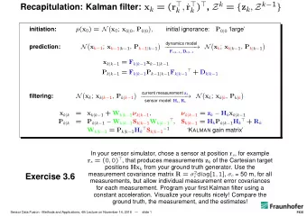
Kalman Filters 16 ● Modelling systems described by a set of continuous variables, e.g., tracking a bird flying— X t = X,Y,Z, ˙ X, ˙ Y , ˙ Z . Airplanes, robots, ecosystems, economies, chemical plants, planets, ... ( Z t = observed position) ● Gaussian prior, linear Gaussian transition model and sensor model Philipp Koehn Artificial Intelligence: Markov Decision Processes 11 April 2017
Updating Gaussian Distributions 17 ● Prediction step: if P ( X t ∣ e 1 ∶ t ) is Gaussian, then prediction P ( X t + 1 ∣ e 1 ∶ t ) = ∫ x t P ( X t + 1 ∣ x t ) P ( x t ∣ e 1 ∶ t ) d x t is Gaussian. If P ( X t + 1 ∣ e 1 ∶ t ) is Gaussian, then the updated distribution P ( X t + 1 ∣ e 1 ∶ t + 1 ) = α P ( e t + 1 ∣ X t + 1 ) P ( X t + 1 ∣ e 1 ∶ t ) is Gaussian ● Hence P ( X t ∣ e 1 ∶ t ) is multivariate Gaussian N ( µ t , Σ t ) for all t ● General (nonlinear, non-Gaussian) process: description of posterior grows unboundedly as t → ∞ Philipp Koehn Artificial Intelligence: Markov Decision Processes 11 April 2017
Simple 1-D Example 18 ● Gaussian random walk on X –axis, s.d. σ x , sensor s.d. σ z t + σ 2 x ) z t + 1 + σ 2 t + σ 2 µ t + 1 = ( σ 2 t + 1 = ( σ 2 x ) σ 2 z µ t z t + σ 2 x + σ 2 σ 2 t + σ 2 x + σ 2 σ 2 σ 2 z z Philipp Koehn Artificial Intelligence: Markov Decision Processes 11 April 2017
General Kalman Update 19 ● Transition and sensor models: P ( x t + 1 ∣ x t ) = N ( Fx t , Σ x )( x t + 1 ) P ( z t ∣ x t ) = N ( Hx t , Σ z )( z t ) F is the matrix for the transition; Σ x the transition noise covariance H is the matrix for the sensors; Σ z the sensor noise covariance ● Filter computes the following update: = F µ t + K t + 1 ( z t + 1 − HF µ t ) µ t + 1 ( I − K t + 1 )( F Σ t F ⊺ + Σ x ) = Σ t + 1 where K t + 1 =( F Σ t F ⊺ + Σ x ) H ⊺ ( H ( F Σ t F ⊺ + Σ x ) H ⊺ + Σ z ) − 1 is the Kalman gain matrix ● Σ t and K t are independent of observation sequence, so compute offline Philipp Koehn Artificial Intelligence: Markov Decision Processes 11 April 2017
2-D Tracking Example: Filtering 20 Philipp Koehn Artificial Intelligence: Markov Decision Processes 11 April 2017
2-D Tracking Example: Smoothing 21 Philipp Koehn Artificial Intelligence: Markov Decision Processes 11 April 2017
22 dynamic baysian networks Philipp Koehn Artificial Intelligence: Markov Decision Processes 11 April 2017
Dynamic Bayesian Networks 23 ● X t , E t contain arbitrarily many variables in a sequentialized Bayes net Philipp Koehn Artificial Intelligence: Markov Decision Processes 11 April 2017
Recommend
More recommend
Explore More Topics
Stay informed with curated content and fresh updates.











![Kalman Filtering Notes Portions of these notes are adapted from [3], [5], [4], [2], and [1]. What](https://c.sambuz.com/985574/kalman-filtering-notes-s.webp)
