Discrete Time Markov Chains Discrete-Time Markov Chains Books - - PDF document

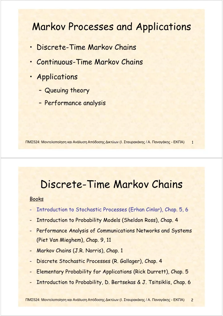
Markov Processes and Applications Markov Processes and Applications • Discrete-Time Markov Chains D k h • Continuous Time Markov Chains • Continuous-Time Markov Chains • Applications Applications – Queuing theory – Performance analysis 1 ΠΜΣ 524: Μοντελοποίηση και Ανάλυση Απόδοσης Δικτύων ( Ι . Σταυρακάκης / Α . Παναγάκης - ΕΚΠΑ ) Discrete Time Markov Chains Discrete-Time Markov Chains Books - Introduction to Stochastic Processes (Erhan Cinlar), Chap. 5, 6 - Introduction to Probability Models (Sheldon Ross) Chap 4 Introduction to Probability Models (Sheldon Ross), Chap. 4 - Performance Analysis of Communications Networks and Systems (Piet Van Mieghem), Chap. 9, 11 - Markov Chains (J.R. Norris), Chap. 1 - Discrete Stochastic Processes (R. Gallager), Chap. 4 - Elementary Probability for Applications (Rick Durrett) Chap 5 Elementary Probability for Applications (Rick Durrett), Chap. 5 - Introduction to Probability, D. Bertsekas & J. Tsitsiklis, Chap. 6 2 ΠΜΣ 524: Μοντελοποίηση και Ανάλυση Απόδοσης Δικτύων ( Ι . Σταυρακάκης / Α . Παναγάκης - ΕΚΠΑ )

INTRODUCTION : th order pdf of some stoc. proc. { p p { } } is given by g y n X t t = ( , ,..., ) ( | , ,..., ) ( | , ,..., ) f x x x f x x x x f x x x x t t t t t t t t t t t − − − − 1 2 1 1 1 2 3 1 n n n n n n n ... ( | ) ( ) f x x f x t t t t t t 2 2 1 1 1 1 very difficult to have it in general • If { } is an indep. process: X t = ( , ,..., ) ( ) ( )... ( ) f x x x f x f x f x t t t t t t − 1 2 1 1 n n n • If { } is a process with indep. increments: X t = − − ( , ,..., ) ( ) ( )... ( ) f x x x f x f x x f x x t t t t t t t t 1 2 1 2 1 − 1 n n n : First order pdf's are sufficient for a bove special cases Note • If { } is a process whose evolution beyond is (probabilistically) X t 0 t < completely determined by and is indep. of , , given , then: x x t t x 0 t t t 0 0 = ( , ,..., ) ( | )... ( | ) ( ) f x x x f x x f x x f x t t t t t t t t − 1 2 1 2 1 1 n n n This is a Markov process ( th order pdf simplified) n 3 ΠΜΣ 524: Μοντελοποίηση και Ανάλυση Απόδοσης Δικτύων ( Ι . Σταυρακάκης / Α . Παναγάκης - ΕΚΠΑ ) Definition of a Markov Process (MP) Definition of a Markov Process (MP) ∈ ∈ A A stoch. stoch proc. proc { { ; ; } } that take that take s s values values from from a a set set is is called called X X t t I I E E t a Markov Process (MP) iff : = = ( ( | | ,..., ) ) ( ( | | ) ) ( ( countable) countable) f f x x x x x x P P x x x x E E t t t t t − 1 1 − 1 n n n n or = ( ( | | ,..., ) ) ( ( | | ) ) ( ( uncountabl uncountabl e) e) f f x x x x x x f f x x x x E E t t t t t − − 1 1 1 n n n n < < < > for all and all ... and all 0 . x t t t n 1 2 t n n : The " next" state is indep. of the " past" { ,..., } Notice x x x t t t − 1 2 n n provided that the " present" is known. 4 ΠΜΣ 524: Μοντελοποίηση και Ανάλυση Απόδοσης Δικτύων ( Ι . Σταυρακάκης / Α . Παναγάκης - ΕΚΠΑ )

Definition of a Markov Chain (MC) (Discrete - time & discrete - value MP) If is countable and is countable then a MP is called a MC I E and d i is d described ib d by the b th transitio t iti n probabilit b bilit ies i : = = = ∈ ( , ) { | } , p i j P X j X i i j E + 1 n n = (indep. ( p of for a time - homogeneou g s MC). ) Assume { { 0 , , 1 , , 2 , } ,...} (state ( - space p of the MC) ) n E Transition matrix : ⎡ ⎡ ⎤ ⎤ ( 0 , 0 ) ( 0 , 1 ) ... ( 0 , ) ... P P P n ⎢ ⎥ ( 1 , 0 ) ( 1 , 1 ) ... ( 1 , ) ... P P P n ⎢ ⎥ ⎢ ⎢ ⎥ ⎥ = = M M M M M M P P ⎢ ⎥ ( , 0 ) ( , 1 ) ... ( , ) ... P n P n P n n ⎢ ⎥ ⎢ ⎥ ⎣ M M M ⎦ ∑ = ∀ is non - negative, ( , ) 1 , i (stochasti c matrix) P P i j j For o a a given g ve (stoc . (stoch. matrix) at ) a a MC C may ay be be constructe co st ucte d d P 5 ΠΜΣ 524: Μοντελοποίηση και Ανάλυση Απόδοσης Δικτύων ( Ι . Σταυρακάκης / Α . Παναγάκης - ΕΚΠΑ ) Chain rule : π π π π = = ∈ ∈ If If is is a a PMF PMF on on s.t. s t ( ( ) ) { { } } , , then then E E i i P P X X i i i i E E 0 0 = = = = = π { , , ,..., } ( ) ( , )... ( , ) P X i X i X i X i i P i i P i i − 0 0 1 1 2 2 0 0 1 1 n n n n ∀ ∀ ∈ ∈ ∈ ∈ , , ,..., n n N N i i i i i i E E 0 1 n k - step transition s : ∀ ∀ ∈ N N , k k = = = { | } ( , ) k P X j X i P i j + n k n ∀ ∈ ∀ ∈ , , N ; ( , ) is the ( , ) entry of the th power k i j E k P i j i j k of the transitio n matrix . P = Proof : For 3 (general through iterations ) k n ∑ ∑ ∑ ∑ = = = { | } ( , ) ( , ) ( , ) P X j X i P i l P l l P l j + 3 1 1 2 2 n n ∈ ∈ l E l E 1 4 4 4 2 4 4 4 3 1 2 2 ( , ) 1 4 4 4 4 4 2 4 P 4 l 4 j 4 4 3 1 3 3 ( , ) P i j 6 ΠΜΣ 524: Μοντελοποίηση και Ανάλυση Απόδοσης Δικτύων ( Ι . Σταυρακάκης / Α . Παναγάκης - ΕΚΠΑ )

Chapman Kolmogorov Equations : From previous, ∑ + = ∈ ( , ) ( , ) ( , ) , m n m n P i j P i k P k j i j E ∈ k E + In order for { } to be in after steps and starting from , X j m n i n it will have to be in some after steps and move then t o in k m j the remaining steps. n 7 ΠΜΣ 524: Μοντελοποίηση και Ανάλυση Απόδοσης Δικτύων ( Ι . Σταυρακάκης / Α . Παναγάκης - ΕΚΠΑ ) siklis ekas & Tsits Bertse 8 ΠΜΣ 524: Μοντελοποίηση και Ανάλυση Απόδοσης Δικτύων ( Ι . Σταυρακάκης / Α . Παναγάκης - ΕΚΠΑ )

# of successes in Bernoulli process Example : ≥ = { { ; 0} } , # of successes in trials f i i l N n N n n n n ∑ ∑ = ≥ = = , 0 , indep. Bernoulli, { 1} N Y n Y P Y p n i i i = 0 i = + ⇒ Notice: evolution of { } beyond N N Y N n + + 1 1 n n n n − 1 does not depe does not depe nd on { nd on { } } n (given (given ) and thus { ) and thus { } is a M C } is a M.C. N N N N N N = 0 i i n n = = = = = = − − { { | | , ,..., } } { { | | , ,..., } } P N P N j N j N N N N N P Y P Y j j N N N N N N N N + + 1 0 1 1 0 1 n n n n n ⎡ ⎤ 0 ... q p = + ⎧ if 1 p j N ⎢ ⎥ n ⎪ ⎪ 0 0 0 0 ... q q p p ⎢ ⎢ ⎥ ⎥ = = − = = 1 if and ⎨ q p j N P ⎢ ⎥ n 0 0 0 ... ⎪ q p 0 otherwise ⎢ ⎥ ⎩ ⎣ ⎣ M M ⎦ ⎦ Notice: { } is a special M.C. whose increment is indep. N n both from present and past (process with indep. increments) p p (p p ) 9 ΠΜΣ 524: Μοντελοποίηση και Ανάλυση Απόδοσης Δικτύων ( Ι . Σταυρακάκης / Α . Παναγάκης - ΕΚΠΑ ) p k = : Sum of i.i.d. RV's with PMF { ; 0,1,2,...} Example k = ⎧ 0 0 n = ⎨ X + + + ≥ n ... 1 ⎩ ⎩ 1 Y Y Y n 1 2 2 n n = = + + X X X X Y Y + + 1 1 n n n = = = − = { | ,..., } { | ,..., } P X j X X P Y j X X X p + + − 1 0 1 0 n n n n n j X n = = = = Thus { Th { } i } is a M.C. with ( , ) M C i h ( ) { { | | } } X X P i j P P X P X j X X i p + − 1 n n n j i ⎡ ⎤ ... p p p p 0 1 2 3 ⎢ ⎢ ⎥ ⎥ 0 ... p p p ⎢ ⎥ 0 1 2 ⎢ ⎥ P = 0 0 ... p p p p 0 0 1 1 ⎢ ⎢ ⎥ ⎥ 0 0 0 ... p ⎢ ⎥ 0 ⎢ ⎥ ⎣ ⎣ M M M M M M M M O O ⎦ ⎦ 10 ΠΜΣ 524: Μοντελοποίηση και Ανάλυση Απόδοσης Δικτύων ( Ι . Σταυρακάκης / Α . Παναγάκης - ΕΚΠΑ )