Stochastic Processes Markov Processes Hamid R. Rabiee 1 Overview - PowerPoint PPT Presentation
Stochastic Processes Markov Processes Hamid R. Rabiee 1 Overview o Markov Property o Markov Chains o Definition o Stationary Property o Paths in Markov Chains o Classification of States o Steady States in MCs. Stochastic Processes 2 Markov
Stochastic Processes Markov Processes Hamid R. Rabiee 1
Overview o Markov Property o Markov Chains o Definition o Stationary Property o Paths in Markov Chains o Classification of States o Steady States in MCs. Stochastic Processes 2
Markov Property A discrete process has the Markov property if given its • value at time t, the value at time t+1 is independent of values at times before t. That is: 𝑄𝑠 𝑌 $%& = 𝑦 $%& 𝑌 $ = 𝑦 $ , 𝑌 $*& = 𝑦 $*& , … , 𝑌 & = 𝑦 & = 𝑄𝑠 𝑌 $%& = 𝑦 $%& 𝑌 $ = 𝑦 $ For all t, x -%& , x - , 𝑦 $*& , 𝑦 $*. , … , 𝑦 & . 3
Stationary Property A Markov Process is called stationary if • Pr 𝑌 $%& = 𝑣|𝑌 $ = 𝑤 = 𝑄𝑠 𝑌 & = 𝑣| 𝑌 0 = 𝑤 for all t. The evolution of stationary processes don’t change over • time. For defining the complete joint distribution of a • stationary Markov Process it is sufficient to define 𝑄𝑠 𝑌 & = 𝑣| 𝑌 0 = 𝑤 and 𝑄𝑠 𝑌 0 = 𝑤 for all u and v. We will mainly consider stationary Markov processes • here. 4
Example (Coin Tossing Game) Consider a single player game in which at every step a • biased coin is tossed and according to the result, the score will be increased or decreased by one point. The game ends if either the score reaches 100 • (winning) or -100 (losing). Score of the player at each step 𝑢 ≥ 0 is a random • variable and the sequence of scores as the game progresses forms a random process 𝑌 7 , 𝑌 & , … , 𝑌 $ . 5
Example (Coin Tossing Game) It is easy to verify that X is a stationary Markov chain: • At the end of each step the score solely depends on the current score 𝑡 9 and the result of tossing the coin (which is independent of time and previous tosses). Stating this mathematically (for 𝑡 9 ∉ {−100,100} ): • 𝑄𝑠 𝑌 $%& = 𝑡 𝑌 $ = 𝑡 9 , 𝑌 $*& = 𝑡 $*& , … , 𝑌 7 = 0 𝑞 ; 𝑡 = 𝑡 9 + 1 Independent of t = ? 1 − 𝑞 ; 𝑡 = 𝑡 9 − 1 and 𝑡 7 , … , 𝑡 $*& 0 ; 𝑝𝑢ℎ𝑓𝑠𝑥𝑗𝑡𝑓 = 𝑄𝑠 𝑌 $%& = 𝑡 𝑌 $ = 𝑡 9 = 𝑄𝑠 𝑌 & = 𝑡 𝑌 7 = 𝑡 9 If value of p was subject to change in time, the process • would not be stationary. In the formulation we would have 𝑞 $ instead of p . • 6
Example (Tracking) Assume we want to track a target in XY plane, and so we need to • model its movement. Assuming that current position and speed of the target describes • everything about its future movements, we can consider the 4- dimensional state: $ , ̇ 𝑌 $ , ̇ 𝑇 $ = (𝑌 $ , 𝑍 𝑍 $ ) It is common to consider linear relation between 𝑇 $ and 𝑇 $*& with a • Gaussian additive noise: 𝑇 $ = 𝐵 $ 𝑇 $*& + 𝑤 $ ; 𝑤 $ ~𝑂(0, Σ) Or equivalently: 𝑔 S T |S TUV 𝑡 $ 𝑡 $*& = 𝑂(𝑡 $ ; 𝐵 $ 𝑡 $*& , Σ) There exists efficient algorithms to work with these linear- • Gaussian models. 7
Example (Tracking) Considering the kinematics relations of a moving object we • can define linear relation as: 1 0 Δ𝑢 0 0 1 0 Δ𝑢 𝐵 $ = Independent of t (stationary) 0 0 1 0 0 0 0 1 This approach can not model Acceleration • the speed is changed only because of noise. • We can model arbitrary speed change by appropriately • setting the 3 rd and 4 th rows of the matrix at each time. An example of a non stationary Markov process. • • Another approach is to extend the states to 6- dimensions containing ̈ 𝑌 $ and ̈ 𝑍 $ . 8
Example (Speech) A basic model for speech signal considers the value at time • t to be a linear combination of its d previous values with a Gaussian additive noise: \ 𝑇 $ = Y 𝛽 Z 𝑇 $*Z + 𝑤 $ ; 𝑤 $ ~𝑂(0, Σ) Z[& 𝑇 $ is not a Markov process. • 9
Example (Speech) We can make a stationary Markov process by considering • the d-dimensional state 𝑉 $ = 𝑇 $ , 𝑇 $*& … , 𝑇 $*\ _ : 𝑉 $ = 𝐵𝑉 $*& + 𝑤 ` 𝐶 Where: 𝛽 & 𝛽 . ⋯ 𝛽 \ 1 1 0 ⋯ 0 0 0 1 𝐵 = , 𝐶 = ⋮ ⋮ ⋱ 1 0 1 Equivalently: • 𝑔 e T |e TUV 𝑣 $ 𝑣 $*& = 𝑂 𝑣 $ ; 𝐵 $ 𝑣 $*& & , Σ 𝕁 ∀ 1 ≤ 𝑗 ≤ 𝑒 ∶ 𝑣 $ Z*& = 𝑣 $*& Z • Which (𝑦) Z is the 𝑗 th dimension of vector 𝑦 and 𝕁 is the indicator function (used for guaranteeing consistency). • Note that we have repeated 𝑌 $ in d consecutive states of U and there should be no inconsistency between those values. 10
Markov Process Types • Two types of Markov processes based on domain of 𝑌 $ values: • Discrete • Continuous • Discrete Markov processes are called “Markov Chains” (MC). • In this session we will focus on stationary MCs. 11
Transition matrix According to the Markov property and stationary property, • at each time step the process moves according to a fixed transition matrix: 𝑄 𝑌 $%& = 𝑘 𝑌 $ = 𝑗 = 𝑞 Zl Stochastic matrix: Rows sum up to 1 • Double stochastic matrix: Rows and columns sum up to 1 12
State Graph It is convenient to visualize a stationary Markov Chain • with a transition diagram: A node represents a possible value of 𝑌 $ . • At each time t, we say the process is in state 𝑡 if 𝑌 $ =s. • Each edge represents the probability of going from one state • to another (we omit edges with zero weight). We should also specify the vector of initial probabilities 𝜌 • = 𝜌 & , … , 𝜌 n where 𝜌 Z = 𝑄𝑠(𝑌 7 = 𝑗) . So a stationary discrete process could be described as a • person walking randomly on a graph (considering each step to depend only on the state he is currently in). The result path is called a “Random Walk”. • 13
Example The transition diagram of the coin tossing game: • p p p 1 p 1 -99 -100 99 100 -98 1-p 1-p 1-p 1-p 1-p • We modeled winning and losing by states which when we get into, we never get out. • Note that if the process was not stationary we were not able to visualize it in this way: • For example consider the case that p is changing in time. 14
Example (Modeling Weather) • Example: Each day is sunny or rainy. If a day is rainy, the next day is rainy with probability 𝛽 (and sunny with probability 1 − 𝛽 ). If the day is sunny, the next day is rainy with probability 𝛾 (and sunny with probability 1 − 𝛾 ). S = {rainy, sunny}, 𝑄 = 𝛽 1 − 𝛽 𝛾 1 − 𝛾 1 − 𝛾 𝛽 1 − 𝛽 R S 𝛾 15
Paths If the state space is {0,1} we have: • 𝑞𝑠 𝑦 2 = 0 𝑦 0 = 0 = 𝑄𝑠 𝑦 & = 1 𝑦 7 = 0 × 𝑞 𝑦 . = 0 𝑦 & = 1 +𝑄𝑠 𝑦 & = 0 𝑦 7 = 0 × 𝑞 𝑦 . = 0 𝑦 & = 0 (n) as the probability that starting from state i, the Define 𝑞 Zl • process stops at state j after n time steps. (.) = ∑ `[& € 𝑞 Zl 𝑞 Z` 𝑞 `l Stochastic Processes 16
Paths Theorem: • € (n) = Y (n*&) 𝑞 `l 𝑞 Zl 𝑞 Z` `[& • To simplify the notation we define the matrix 𝑄 (n) such that (n) . the value at the i’th row and j’th column is 𝑞 Zl • Corollary 1: 𝑄 (n) can be calculated by: 𝑄 (n) = 𝑄 n Corollary 2: If the process starts at time 0 with distribution • 𝜌 on the states then after n steps the distribution is 𝜌𝑄 n . Stochastic Processes 17
Absorbing Markov Chain An absorbing state is one in which the probability that the • process remains in that state once it enters the state is 1 (i.e., 𝑞 ZZ = 1 ). A Markov chain is absorbing if it has at least one absorbing • state, and if from every state it is possible to go to an absorbing state (not necessarily in one step). An absorbing Markov chain will eventually enter one of the • absorbing states and never leave it. Example: The 100 and -100 states in coin tossing game • Note: After playing ling enough, the player will either win • or lose (with probability 1). p p p 1 p 1 -99 100 -100 99 -98 1-p 1-p 1-p 1-p 1-p Stochastic Processes 18
Absorption theorem In an absorbing Markov chain the probability that the • process will be absorbed is 1. Proof: From each non-absorbing state 𝑡 l it is possible to • reach an absorbing state starting from 𝑡 l . Therefore there exists p and m, such that the probability of not absorbing after m steps is at most p, in 2m steps at most 𝑞 . , etc. Since the probability of not being absorbed is • monotonically decreasing, we have: n→„ Pr(not absorbed after n steps) =0 lim • Stochastic Processes 19
Classification of States Accessibility: State j is said to be accessible from state i if • starting in i it is possible that the process will ever enter state j: (𝑄 n ) Zl > 0 . Communication: Two states i and j that are accessible to each • other are said to communicate. Every node communicates with itself: • 7 = Pr 𝑌 7 = 𝑗 𝑌 7 = 𝑗 = 1 • p †† Communication is an equivalence relation: It divides the • state space up into a number of separate classes in which every pair of states communicate. (why?) The Markov chain is said to be irreducible if it has only one • class. Stochastic Processes 20
Recommend
More recommend
Explore More Topics
Stay informed with curated content and fresh updates.
