Discrete time Markov chains Today: Discrete Time Markov Chains, - PowerPoint PPT Presentation
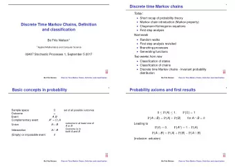
Discrete time Markov chains Today: Discrete Time Markov Chains, Limiting Discrete time Markov chains - invariant probability Distribution and Classification distribution Classification of states Classification of chains Bo Friis
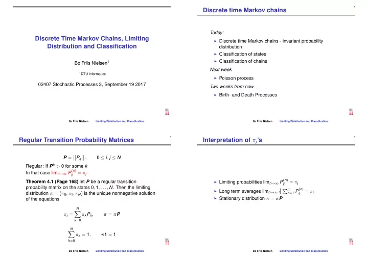
Discrete time Markov chains Today: Discrete Time Markov Chains, Limiting ◮ Discrete time Markov chains - invariant probability Distribution and Classification distribution ◮ Classification of states ◮ Classification of chains Bo Friis Nielsen 1 Next week 1 DTU Informatics ◮ Poisson process 02407 Stochastic Processes 3, September 19 2017 Two weeks from now ◮ Birth- and Death Processes Bo Friis Nielsen Limiting Distribution and Classification Bo Friis Nielsen Limiting Distribution and Classification Regular Transition Probability Matrices Interpretation of π j ’s � , � �� � �� P = � P ij 0 ≤ i , j ≤ N Regular: If P k > 0 for some k In that case lim n →∞ P ( n ) = π j ij ◮ Limiting probabilities lim n →∞ P ( n ) Theorem 4.1 (Page 168) let P be a regular transition = π j ij probability matrix on the states 0 , 1 , . . . , N . Then the limiting n = 1 P ( n ) ◮ Long term averages lim n →∞ 1 � m = π j distribution π = ( π 0 , π 1 , π N ) is the unique nonnegative solution 1 ij ◮ Stationary distribution π = π P of the equations N � π j = π k P ij , π = π P k = 0 N � π k = 1 , π 1 = 1 k = 0 Bo Friis Nielsen Limiting Distribution and Classification Bo Friis Nielsen Limiting Distribution and Classification
A Social Mobility Example Classification of Markov chain states Son’s Class ◮ States which cannot be left, once entered - absorbing Lower Middle Upper states Lower 0.40 0.50 0.10 ◮ States where the return some time in the future is certain - Father’s Middle 0.05 0.70 0.25 recurrent or persistent states Class Upper 0.05 0.50 0.45 ◮ The mean time to return can be ◮ finite - postive recurrence/non-null recurrent � � � � 0 . 0772 0 . 6250 0 . 2978 ◮ infinite - null recurrent � � � � P 8 = � � � � 0 . 0769 0 . 6250 0 . 2981 � � � � ◮ States where the return some time in the future is � � � � 0 . 0769 0 . 6250 0 . 2981 � � � � uncertain - transient states ◮ States which can only be visited at certain time epochs - π 0 = 0 . 40 π 0 + 0 . 05 π 1 + 0 . 05 π 2 periodic states π 1 = 0 . 50 π 0 + 0 . 70 π 1 + 0 . 50 π 2 π 2 = 0 . 10 π 0 + 0 . 25 π 1 + 0 . 45 π 2 1 = π 0 + π 1 + π 2 Bo Friis Nielsen Limiting Distribution and Classification Bo Friis Nielsen Limiting Distribution and Classification Classification of States First passage and first return times We can formalise the discussion of state classification by use of a certain class of probability distributions - first passage time distributions. Define the first passage probability f ( n ) = P { X 1 � = j , X 2 � = j , . . . , X n − 1 � = j , X n = j | X 0 = i } ij ◮ j is accessible from i if P ( n ) > 0 for some n ij This is the probability of reaching j for the first time at time n ◮ If j is accessible from i and i is accessible from j we say having started in i . that the two states communicate What is the probability of ever reaching j ? ◮ Communicating states constitute equivalence classes (an equivalence relation) ∞ f ( n ) ◮ i communicates with j and j communicates with k then i � f ij = ≤ 1 ij and k communicates n = 1 The probabilities f ( n ) constitiute a probability distribution. On ij n = 1 p ( n ) the contrary we cannot say anything in general on � ∞ ij (the n -step transition probabilities) Bo Friis Nielsen Limiting Distribution and Classification Bo Friis Nielsen Limiting Distribution and Classification
State classification by f ( n ) Classification of Markov chains ii � � n = 1 f ( n ) ◮ A state is recurrent (persistent) if f ii = � ∞ = 1 ii ◮ A state is positive or non-null recurrent if E ( T i ) < ∞ . n = 1 nf ( n ) ◮ We can identify subclasses of states with the same E ( T i ) = � ∞ = µ i ii ◮ A state is null recurrent if E ( T i ) = µ i = ∞ properties ◮ A state is transient if f ii < 1. ◮ All states which can mutually reach each other will be of In this case we define µ i = ∞ for later convenience. the same type ◮ A peridoic state has nonzero p ii ( nk ) for some k . ◮ Once again the formal analysis is a little bit heavy, but try to stick to the fundamentals, definitions (concepts) and results ◮ A state is ergodic if it is positive recurrent and aperiodic. Bo Friis Nielsen Limiting Distribution and Classification Bo Friis Nielsen Limiting Distribution and Classification Properties of sets of intercommunicating states A set C of states is called ◮ (a) Closed if p ij = 0 for all i ∈ C , j / ∈ C ◮ (b) Irreducible if i ↔ j for all i , j ∈ C . Theorem Decomposition Theorem The state space S can be partitioned ◮ (a) i and j has the same period uniquely as ◮ (b) i is transient if and only if j is transient S = T ∪ C 1 ∪ C 2 ∪ . . . ◮ (c) i is null persistent (null recurrent) if and only if j is null where T is the set of transient states, and the C i are irreducible persistent closed sets of persistent states � Lemma If S is finite, then at least one state is persistent(recurrent) and all persistent states are non-null (positive recurrent) � Bo Friis Nielsen Limiting Distribution and Classification Bo Friis Nielsen Limiting Distribution and Classification
Basic Limit Theorem An example chain (random walk with reflecting barriers) Theorem 4.3 The basic limit theorem of Markov chains 0 . 6 0 . 4 0 . 0 0 . 0 0 . 0 0 . 0 0 . 0 0 . 0 (a) Consider a recurrent irreducible aperiodic Markov 0 . 3 0 . 3 0 . 4 0 . 0 0 . 0 0 . 0 0 . 0 0 . 0 chain. Let P ( n ) be the probability of entering state i ii 0 . 0 0 . 3 0 . 3 0 . 4 0 . 0 0 . 0 0 . 0 0 . 0 at the n th transition, n = 1 , 2 , . . . , given that 0 . 0 0 . 0 0 . 3 0 . 3 0 . 4 0 . 0 0 . 0 0 . 0 X 0 = i . By our earlier convention P ( 0 ) = 1. Let f ( n ) P = ii ii 0 . 0 0 . 0 0 . 0 0 . 3 0 . 3 0 . 4 0 . 0 0 . 0 be the probability of first returning to state i at the 0 . 0 0 . 0 0 . 0 0 . 0 0 . 3 0 . 3 0 . 4 0 . 0 n th transition n = 1 , 2 , . . . , where f ( 0 ) = 0. Then 0 . 0 0 . 0 0 . 0 0 . 0 0 . 0 0 . 3 0 . 3 0 . 4 ii 0 . 0 0 . 0 0 . 0 0 . 0 0 . 0 0 . 0 0 . 3 0 . 7 1 = 1 n →∞ P ( n ) lim = With initial probability distribution p ( 0 ) = ( 1 , 0 , 0 , 0 , 0 , 0 , 0 , 0 ) or ii n = 0 nf ( n ) m i � ∞ ii X 0 = 1. (b) under the same conditions as in (a), lim n →∞ P ( n ) = lim n →∞ P ( n ) for all j . ji ii Bo Friis Nielsen Limiting Distribution and Classification Bo Friis Nielsen Limiting Distribution and Classification Properties of that chain A number of different sample paths X n ’s ◮ We have a finite number of states ◮ From state 1 we can reach state j with a probability 8 8 f 1 j ≥ 0 . 4 j − 1 , j > 1. 7 7 6 6 5 5 ◮ From state j we can reach state 1 with a probability 4 4 3 3 f j 1 ≥ 0 . 3 j − 1 , j > 1. 2 2 1 1 0 10 20 30 40 50 60 70 0 10 20 30 40 50 60 70 ◮ Thus all states communicate and the chain is irreducible. Generally we won’t bother with bounds for the f ij ’s. ◮ Since the chain is finite all states are positive recurrent 8 8 ◮ A look on the behaviour of the chain 7 7 6 6 5 5 4 4 3 3 2 2 1 1 0 10 20 30 40 50 60 70 0 10 20 30 40 50 60 70 Bo Friis Nielsen Limiting Distribution and Classification Bo Friis Nielsen Limiting Distribution and Classification
Limiting distribution The state probabilities For an irreducible aperiodic chain, we have that → 1 p ( n ) as n → ∞ , for all i and j ij µ j 1 0.9 0.8 Three important remarks 0.7 0.6 ◮ If the chain is transient or null-persistent (null-recurrent) 0.5 0.4 p ( n ) → 0 0.3 ij 0.2 ◮ If the chain is positive recurrent p ( n ) → 1 0.1 ij 0 µ j 0 10 20 30 40 50 60 70 ◮ The limiting probability of X n = j does not depend on the starting state X 0 = i p ( n ) j Bo Friis Nielsen Limiting Distribution and Classification Bo Friis Nielsen Limiting Distribution and Classification The stationary distribution Stationary distribution Definition The vector π is called a stationary distribution of the chain if π has entries ( π j : j ∈ S ) such that ◮ A distribution that does not change with n ◮ (a) π j ≥ 0 for all j , and � j π j = 1 ◮ The elements of p ( n ) are all constant ◮ (b) π = π P , which is to say that π j = � i π i p ij for all j . ◮ The implication of this is p ( n ) = p ( n − 1 ) P = p ( n − 1 ) by our � assumption of p ( n ) being constant VERY IMPORTANT An irreducible chain has a stationary distribution π if and only if ◮ Expressed differently π = π P all the states are non-null persistent (positive recurrent);in this case, π is the unique stationary distribution and is given by π i = 1 µ i for each i ∈ S , where µ i is the mean recurrence time of i . Bo Friis Nielsen Limiting Distribution and Classification Bo Friis Nielsen Limiting Distribution and Classification
Recommend
More recommend
Explore More Topics
Stay informed with curated content and fresh updates.
