Markov Chains Markov Processes Discrete-time Markov Chains - - PowerPoint PPT Presentation

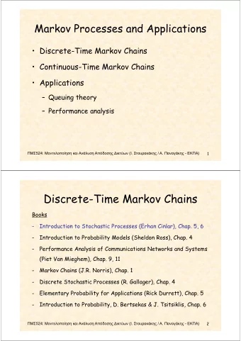
Markov Chains

Markov Processes Discrete-time Markov Chains Continuous-time Markov Chains

Dr Conor McArdle EE414 - Markov Chains 1/30

Markov Processes

A Markov Process is a stochastic process Xt with the Markov property: Pr(Xtn ≤ xn | Xtn−1 = xn−1, Xtn−2 = xn−2, ... , Xt0 = x0) = Pr(Xtn ≤ xn | Xtn−1 = xn−1) ∀ states xi in the process’ state space S ∀ times t0 ≤ t1... ≤ tn ∈ R+ That is, the distribution of the possible states (values) of the Markov process at a time tn (i.e. the cdf of Xtn) is dependent only on the previous state of the process xn−1 at a time tn−1, and is independent of the whole history of states previous to that. Equivalently, we can say that the states of a Markov process previous to the current state of the process have no effect on determining the future path of the process. Markov processes are very useful for analysing the performance of a wide range of computer and communications system. These processes are relatively easy to solve, given the simplified form of the joint distribution function.

Dr Conor McArdle EE414 - Markov Chains 2/30

Markov Processes: Time-homogeneity

In general, the distribution Pr(Xtn ≤ xn | Xtn−1 = xn−1), governing the probabilities of the occurrence of different values of the process, is not only dependent on the value of the last previous state, xn−1, but is also dependent on the current time tn at which we

• bserve the process to be in state xn and the time tn−1 at which is was previously
• bserved to be in state xn−1.

For the Markov processes of interest in this course, we may always assume that this time dependence is limited to a dependence on the difference of the times tn and tn−1. Such Markov processes are referred to as time homogeneous or simply homogeneous. A Markov process is said to be time-homogeneous if Pr(Xtn ≤ xn | Xtn−1 = xn−1) = Pr(Xtn−tn−1 ≤ xn | X0 = xn−1) ∀n Note that time homogeneity and stationarity are not the same concept. For a stationary process the (unconditinal) cdf does not change with shifts in time. For a homogeneous process, the conditional cdf of Xtn does not change with shifts in time. That is, a homogeneous process is not necessarily a stationary process.

Dr Conor McArdle EE414 - Markov Chains 3/30

Markov Processes: Markov Chains

Markov processes may be further classified according to whether the state space and/or parameter space (time) are discrete or continuous. A Markov process which has a discrete state space (with either discrete or continuous parameter spaces) is referred to as as a Markov Chain. For a Markov Chain, we write the Markov property in terms of a state’s conditional pmf (as opposed to conditional cdf for a continuous state space): For a continuous-time Markov Chain we write: Pr(Xtn = j | Xtn−1 = in−1, Xtn−2 = in−2, ... , Xt0 = i0) = Pr(Xtn = j | Xtn−1 = in−1) ∀ j ∈ S, ∀ i0, i1, ... ∈ S, ∀ t0 ≤ t1... ≤ tn ∈ R+ For a discrete-time Markov Chain we write: Pr(Xn = j | Xn−1 = in−1, Xn−2 = in−2, ... , X0 = i0) = Pr(Xn = j | Xn−1 = in−1) ∀ j ∈ S, ∀ i0, i1, ... ∈ S, ∀ n ∈ N In either case, the process ranges over a discrete states space S. This state space may be finite or (countably) infinite.

Dr Conor McArdle EE414 - Markov Chains 4/30

Markov Processes: Example

Consider a game where a coin is tossed repeatedly and the player’s score is accumulated by adding 2 points when a head turns up and adding 1 point for a tail. Is this a Markov Chain? Is the process homogeneous? The state space of the process is formed by all possible accumulated scores that can

• ccur over the course of the game (i.e. S = N). For any given state we see that the

distribution of possible values of the state is dependent only on the previous state, that is, the state distribution is described by: Pr(Xn = j + 1 | Xn−1 = j) = 1 2 Pr(Xn = j + 2 | Xn−1 = j) = 1 2 and thus the process is a Markov process. Also, the state space is discrete (countably infinite), so the process is a Markov Chain. Further more, the distribution of possible values of a state does not depend upon the time the observation is made, so the process is a homogeneous, discrete-time, Markov Chain.

Dr Conor McArdle EE414 - Markov Chains 5/30

Markov Chains & Birth-Death Processes

Markov Processes Discrete-time Markov Chains Continuous-time Markov Chains

Dr Conor McArdle EE414 - Markov Chains 6/30

Discrete-time Markov Chains

We have defined a discrete-time Markov Chain as a process having the property Pr(Xn = j | Xn−1 = in−1, Xn−2 = in−2, ... , X0 = i0) = Pr(Xn = j | Xn−1 = in−1) ∀ j ∈ S, ∀ i0, i1, ... ∈ S, ∀ n ∈ N We say that when Xn = j, the process is observed to be in state j at time n. Pr(Xn = j | Xn−1 = i) is the probability of finding the process in state j at time instance n (step n of the process), given that the system was previously in state i at time instance (step) n − 1. Equivalently, we can say that Pr(Xn = j | Xn−1 = i) is the probability of the process transitioning from state i into state j (in a single step) at time instance n. This probability is called the one-step transition probability, denoted as pij(n). As we will always assume homogeneity, Pr(Xn = j | Xn−1 = i) is the same probability for any n and so pij(n) is independent of n and the one-step transition probability is: pij P[Xn = j | Xn−1 = i], ∀n

Dr Conor McArdle EE414 - Markov Chains 7/30

Discrete-time Markov Chains: Transition Probabilities

The set of all transition probabilities pij for all i and all j may be expressed in matrix form as a transition probability matrix P where: P =      p0,0 p0,1 p0,2 . . . p1,0 p1,1 p1,2 . . . p2,0 p2,1 p2,2 . . . . . . . . . . . . ...      The ith row of P are the probabilities of transitioning out of state i to other states of the process (including back to state i). The sum of these probabilities is the probability of transitioning to some other state from i and so must equal 1, i.e.

• ∀j

pi,j = 1. The jth column of P are the probabilities of transitioning from states of the process (including state j) into state j. The sum of these probabilities is generally = 1. Exercise 7: Again, consider the game where a coin is tossed repeatedly and the player’s score is accumulated by adding 2 points when a head turns up and adding 1 point for a tail. Write down the transition probability matrix P for the process.

Dr Conor McArdle EE414 - Markov Chains 8/30

Discrete-time Markov Chains: Transition Probabilities

We may calculate the probability of a transition from a state i to a state j in two steps, through a given intermediate state k, as pik pkj. This is true as, by the Markov property, the transitions i → k and k → j are independent events. Additionally, by applying the Law of Total Probability, P[A] =

∀i P(Bi)P(A | Bi), the

probability of transitioning from i to j in two steps through any intermediate state k may be calculated as: p(2)

ij =

• ∀k

pik pkj Furthermore, we may calculate the m-step transition probability from state i to state j recursively: p(m)

ij

=

• ∀k

p(m−1)

ik

pkj m = 2, 3, . . . This equation is called the Chapman-Kolmogorov Equation. It is a fundamental equation in the analysis of Markov chains, allowing us to calculate of the probability that the process is in a particular state after m time steps.

Dr Conor McArdle EE414 - Markov Chains 9/30

Discrete-time Markov Chains: Transition Probabilities

We may express the Chapman-Kolmogorov equation in a more compact matrix form by noting that the element {i, j} of the matrix P.P = P2 is equal to

∀k pik pkj, which

is equal to the two-step transition probability p(2)

ij .

Similarly, the element {i, j} of Pm is equal to the m-step transition probability p(m)

ij .

Thus, we can express the Chapman-Kolmogorov Equation as: Pm = Pm−1P

• r alternatively, in a more general form, as:

Pm = Pm−nPn Pm is referred to as the m-step transition probability matrix of the Markov chain. We now consider how the probability of being in a particular state at a particular time may be calculated from Pm.

Dr Conor McArdle EE414 - Markov Chains 10/30

Discrete-time Markov Chains: State Probabilities

We denote the probability of the process being in state i at step n as: π(n)

i

= Pr(Xn = i) We refer to this as a state probability. The state probabilities for all states at step n may be expressed as a state distribution vector π(n) = (π(n)

0 , π(n) 1 , π(n) 2 , . . .)

Applying the Law of Total Probability, the probability that the process is in state i at time step 1 may be calculated as: π(1)

i

=

• ∀k

π(0)

k pki

Or equivalently, in vector-matrix notation, the state distribution vector at the first step may be expressed as: π(1) = π(0)P π(0) is referred to as the initial state distribution. It is an arbitrarily chosen distribution of the starting state of the process at time step 0.

Dr Conor McArdle EE414 - Markov Chains 11/30

Discrete-time Markov Chains: State Probabilities

The calculation of state probabilities can be continued for successive steps, as follows: π(1) = π(0)P π(2) = π(1)P = [π(0)P]P = π(0)P2 . . . π(n) = π(n−1)P = π(0)Pn n = 1, 2, 3, . . . This gives us an important result for Markov chain analysis. Knowing the initial distribution of states π(0) at time step 0, and the transition probabilities between states given by P, we can calculate the distribution of states (the probability of being in any particular state) at any future time step n. π(n) = π(0)Pn n = 1, 2, 3, . . .

Dr Conor McArdle EE414 - Markov Chains 12/30

Discrete-time Markov Chains: State Probabilities

Exercise 8 Yet again, consider the game where a coin is tossed repeatedly and the player’s score is accumulated by adding 2 points when a head turns up and adding 1 point for a tail. We have previously found the transition probability matrix P for the process. By using the fact that π(n) = π(0)Pn, n = 1, 2, 3, . . ., calculate the probability that the player’s score is at least 4 points having tossed the coin 3 times.

Dr Conor McArdle EE414 - Markov Chains 13/30

Discrete-time Markov Chains: State Probabilities and Equilibrium

We have found a method to calculate π(n), which encodes the probable evolution of the Markov Chain over time starting at time 0. This vector is referred to as the transient solution of the Markov Chain. We are also interested in how a Markov Chain behaves after a long time period (after many steps). We can see that a process’s state distribution changes for successive steps starting at time 0. However, does a process’s state distribution ‘settle down’ over time to an equilibrium solution, that is, is there a limiting stationary distribution of the states after a long time period? Can we thus calculate the expected value of the process? It is important to answer these questions so that we can take the analysis further and to calculate useful parameters of stochastic processes arising in communications performance analysis. Exercise 9 Would you expect the process in the previous example to have a stationary dis- tribution as n → ∞? Is the process ergodic (as per the definition given in the Stochastic Processes section)?

Dr Conor McArdle EE414 - Markov Chains 14/30

Discrete-time Markov Chains: Classifications

To find the conditions under which a stationary distribution exists, we must first define some general properties of Markov Chains: Closure A subset of the states A is closed if there is no possible transition from any state in A to any state in AC. Absorption A single state which is a closed set is called an absorbing state. That is, it is not possible to transition out of an absorbing state i (pii = 1). Reducibility A closed set of states is called irreducible if it contains no closed (proper) subsets of

• itself. A Markov Chain is irreducible if the set of all state is irreducible.

An alternative definition is that a Markov Chain is irreducible if every state can be reached from every other state. That is, for all states i and j, there is an integer m such that p(m)

ij

> 0. Conversely, a set of states is reducible if there exists a closed, proper subset of itself.

Dr Conor McArdle EE414 - Markov Chains 15/30

Discrete-time Markov Chains: Classifications

Recurrence Further classifications are made based on whether or not, and how often, a state is revisited. Let f(n)

i

be the probability of the first return to state i in exactly n steps (n ≥ 1). The probability of ever returning to state i is fi = ∞

n=1 f(n) i

. The mean recurrence time of state i is Mi = ∞

n=1 n f(n) i

. A state i is said to be transient if the probability of returning to the state is less < 1 (fi < 1). A state i is said to be recurrent if fi = 1. A state i is positive recurrent if its mean recurrence time is finite (Mi < ∞). A state i is null recurrent if its mean recurrence time is infinite (Mi = ∞). Periodicity A i state is periodic if its first return time f(n)

i

can only be a multiple of an integer greater than 1. Otherwise, the state is called aperiodic.

Dr Conor McArdle EE414 - Markov Chains 16/30

Discrete-time Markov Chains: Theorems

Theorem 1 The states of an irreducible Markov Chain are either all transient or all null-recurrent or all positive-recurrent Additionally, all states are either aperiodic or periodic. We are most interested in ’well-behaved’ Markov Chains which have a unique stationary distribution. These types of chains are described as ergodic. Definition: An irreducible Markov Chain which is positive-recurrent and aperiodic is said to be ergodic. The next theorem states that a unique stationary distribution always exists for a homogeneous Markov Chain that is ergodic.

Dr Conor McArdle EE414 - Markov Chains 17/30

Discrete-time Markov Chains: Theorems

Theorem 2 - Kolmogorov’s Theorem In an irreducible, aperiodic, time-homogeneous Markov Chain the limits πj = lim

n→∞ π(n) j

∀ j (1) always exist and are independent of the initial state probability distribution π(0). Moreover, either: (a) all states are transient or all states are null-recurrent in which case πj = 0 for all j and there exists no stationary distribution, or (b) all states are positive-recurrent and then πj > 0 for all j, in which case the set {πj} is a stationary probability distribution and πj = 1 Mj where Mj is the mean recurrence time for state j In this case the quantities πj are uniquely determined by: πj =

• ∀i

πi pij (2) and 1 =

• ∀i

πi (3)

Dr Conor McArdle EE414 - Markov Chains 18/30

Discrete-time Markov Chains: Stationary Distribution

We may re-write (1) above, using our previous vector-matrix notation, as π = lim

n→∞ π(n)

π is the stationary distribution of the Markov Chain, also know as the equilibrium solution or the equilibrium (or steady-state) state probability vector. We may write (2) and (3) using more compact vector/matrix notation as π = πP (2) Called the ’global balance equation’ π.1T = 1 (3) Called the ’normalisation condition’ where 1 is the unit row vector. We note that (2) can be obtained from the state probabilities equation, by way of π(n) = π(n−1)P lim

n→∞ π(n) = lim n→∞ π(n−1)P

π = πP

Dr Conor McArdle EE414 - Markov Chains 19/30

Discrete-time Markov Chains: Example

Example Consider the State Transition Diagram below showing the probabilities of a Markov chain transitioning between its three states. (i) Explain why this chain must have a stationary distribution and (ii) calculate the equilibrium probabilities π. (iii) Calculate the transient solution π(n) for the first four steps of the process (n = 1, 2, 3, 4) for each of the initial state distribution vectors π(0) = (1, 0, 0), π(0) = (0, 1, 0) and π(0) = (0, 0, 1).

3/4 1/4 1/4 3/4 1/4 1/4 1/2 Dublin(1) Limerick(0) Cork(2)

Dr Conor McArdle EE414 - Markov Chains 20/30

Discrete-time Markov Chains: Example

Solution (i) We can see that the process is a homogeneous Markov Chain. It is also irreducible as all states are reachable from any state. It is recurrent as we will surely return to a state over time and is positive-recurrent as the expected first return time is less than

• infinity. Furthermore it is aperiodic. Thus, by Theorem 2, the process must have a

stationary distribution. (ii) From the state transition diagram we have P =  

3 4 1 4 1 4 3 4 1 4 1 4 1 2

  Applying π = πP we have π0 = 0π0 + 1 4π1 + 1 4π2 π1 = 3 4π0 + 0π1 + 1 4π2 π2 = 1 4π0 + 3 4π1 + 1 2π2

Dr Conor McArdle EE414 - Markov Chains 21/30

Discrete-time Markov Chains: Example

In addition, the normalisation condition π.1T = 1 gives π0 + π1 + π2 = 1 We now have a system of four simultaneous equations which must have a unique solution (by Theorem 2). Solving the equations gives the solution: π0 = 1 5 π1 = 7 25 π2 = 13 25

• r in vector notation:

π = 1

5, 7 25, 13 25

• These are the equilibrium state probabilities (the stationary distribution of the Markov

Chain). (iii) We may calculate the transient solution for the first few steps of the process using π(n) = π(n−1)P iteratively, that is: π(1) = π(0)P π(2) = π(1)P π(3) = π(2)P . . .

Dr Conor McArdle EE414 - Markov Chains 22/30

Discrete-time Markov Chains: Example

We do this for the different starting points (the different initial state probabilities) (1, 0, 0), (0, 1, 0) and (0, 0, 1). The results are: n 1 2 3 4 ... ∞ π(n) 1 0.00 0.25 0.19 0.20 0.20 π(n)

1

0.75 0.06 0.36 0.25 0.28 π(n)

2

0.25 0.69 0.45 0.55 0.52 n 1 2 3 4 ... ∞ π(n) 0.25 0.19 0.20 0.20 0.20 π(n)

1

1 0.00 0.38 0.25 0.29 0.28 π(n)

2

0.75 0.43 0.55 0.51 0.52 n 1 2 3 4 ... ∞ π(n) 0.25 0.19 0.20 0.20 0.20 π(n)

1

0.25 0.31 0.27 0.29 0.28 π(n)

2

1 0.50 0.50 0.53 0.51 0.52 We note that after four steps the state distribution vectors are very close in value to the stationary distribution vector, regardless of the starting point of the process.

Dr Conor McArdle EE414 - Markov Chains 23/30

Markov Chains & Birth-Death Processes

Markov Processes Discrete-time Markov Chains Continuous-time Markov Chains

Dr Conor McArdle EE414 - Markov Chains 24/30

Continuous-time Markov Chains

In the case of a continuous-time Markov Chain, state transitions may occur at any arbitrary time instance and not merely at fixed, discrete time points, as was the case for discrete-time chains. Thus, for the continuous-time Markov Chain, the Markov property is expressed in terms of the continuous time parameter t ∈ R+ as Pr(Xtn = j | Xtn−1 = in−1, Xtn−2 = in−2, ... , Xt0 = i0) = Pr(Xtn = j | Xtn−1 = in−1) ∀ j ∈ S, ∀ i0, i1, ... ∈ S, ∀ t0 ≤ t1... ≤ tn ∈ R+ That is, the process is entirely described by the state transition probability Pr(Xtn = j | Xtn−1 = i), the probability of finding the process in state j at a time tn, given that it was in state i at time tn−1, for all i, j, tn−1 and tn. As with the discrete time case, we only concern ourselves with chains that are time-homogeneous. In this case, for any times t1 < t2, and t t2 − t1 Pr(Xt2 = j | Xt1 = i) = Pr(Xt = j | X0 = i) and we denote this transition probability as pij(t) ≡ pij(0, t) = Pr(Xt = j | X0 = i) = Pr(Xt2 = j | Xt1 = i)

Dr Conor McArdle EE414 - Markov Chains 25/30

Continuous-time Markov Chains

pij(0, t) is analogous to the m-step transition probability in the discrete-time case, where the discrete-time variable m is replaced by the continuous-time variable t. Similarly to the discrete-time case, the Chapman-Kolmogorov equation for the continuous-time Markov chain may be written as: pij(t) = pij(0, t) =

• ∀k∈S

pik(0, t′)pkj(t′, t), 0 < t′ < t (4) Or in matrix notation we may write equation (4) as P(t) = P(t′)P(t − t′) If we denote the state probabilities, the probability of being in state i at a time t, as πi(t) = Pr(Xt = i), we may write the relationship between state probabilities and transition probabilities, for the continuous-time Markov chain, as: πj(t) =

• ∀i∈S

pij(t)πi(0) (5) Or in vector-matrix notation we may write equation (5) as π(t) = π(0)P(t) .

Dr Conor McArdle EE414 - Markov Chains 26/30

Continuous-time Markov Chains

In summary, similar to the discrete-time case, we have two equations in terms of the state probability distribution vector π(t) and the transition probability matrix P(t), from which we wish to resolve the transient and steady-state (stationary) state probabilities. As with the discrete-time case, the existence of the stationary distribution of the state probabilities depends on the properties of the chain. We first resolve the transient solution and then examine the steady-state solution. In the discrete-time case pij did not have a dependence on the length of time between state changes and the solution was obtained by solving a set of linear equations. In the continuous-time case, the transition probabilities pij(t) are dependent on t and the solution is more involved. Instead of resolving the probabilities pij(t) directly, we express the probabilities in terms of a quantity qij for which, for time-homogeneous chains, we can remove the dependence on the transition time. qij is termed the state transition rate, the rate at which the chain leaves state i in

• rder to transition in state j.

Dr Conor McArdle EE414 - Markov Chains 27/30

Continuous-time Markov Chains

We define this transition rate as qij lim

∆t→0

pij(t, t + ∆t) ∆t , i = j qii lim

∆t→0

pii(t, t + ∆t) − 1 ∆t Now, considering the Chapman-Kolmogorov equation (4) at time points 0, t and t + ∆t pij(t + ∆t) =

• ∀k∈S

pik(t)pkj(∆t) Dividing by ∆t and taking the limit as ∆t → 0 lim

∆t→0

pij(t + ∆t) ∆t =

• ∀k∈S

pik(t) lim

∆t→0

pkj(∆t) ∆t d dt pij(t) =

• ∀k∈S

pik(t) qkj (6)

Dr Conor McArdle EE414 - Markov Chains 28/30

Continuous-time Markov Chains

Now, differentiating (5) w.r.t. t and then substituting from (6): d dt πj(t) =

• ∀i∈S

d dt pij(t)πi(0) =

• ∀i∈S
• ∀k∈S

pik(t) qkj πi(0) =

• ∀k∈S

qkj

• ∀i∈S

pik(t) πi(0) d dt πj(t) =

• ∀k∈S

qkj πk(t) The solution of this system of differential equations gives the transient solution π = {πi(t)} of the continuous-time (homogeneous) Markov Chain. We can express these equations in vector-matrix form as ˙ π(t) = π(t)Q The structure of Q determines how easy/difficult it is to find a solution for π. Will are most interested in processes called Birth-Death processes, which have a ’nice’ Q matrix that makes the system relatively easy to solve.

Dr Conor McArdle EE414 - Markov Chains 29/30

Continuous-time Markov Chains: Stationary Distribution

Similarly to the discrete-time case, it can be shown that a homogeneous continuous-time chain that is ergodic has a unique stationary (steady-state) distribution π. In this case, π(t) tends to the constant π as t → ∞, so lim

t→∞

d πi(t) d t = 0, ∀i ∈ S which yields a simple set of linear equations for resolving π

• ∀i∈S

qij πi = 0, ∀j ∈ S

• r, in vector-matrix notation, the steady-state solution is given by resolution of

0 = πQ To find a unique solution, we must also impose the normalisation condition π1T =

• ∀i∈S

πi = 1

Dr Conor McArdle EE414 - Markov Chains 30/30