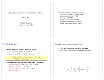
Discrete time Markov chains Today: Short recap of probability - PowerPoint PPT Presentation

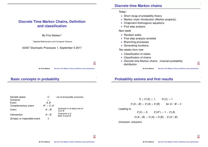
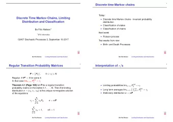
Discrete time Markov chains Today: ◮ Short recap of probability theory ◮ Markov chain introduction (Markov property) Discrete Time Markov Chains, Definition ◮ Chapmann-Kolmogorov equations and classification ◮ First step analysis Next week ◮ Random walks Bo Friis Nielsen 1 ◮ First step analysis revisited 1 Applied Mathematics and Computer Science ◮ Branching processes ◮ Generating functions 02407 Stochastic Processes 1, September 5 2017 Two weeks from now ◮ Classification of states ◮ Classification of chains ◮ Discrete time Markov chains - invariant probability distribution Bo Friis Nielsen Discrete Time Markov Chains, Definition and classification Bo Friis Nielsen Discrete Time Markov Chains, Definition and classification Basic concepts in probability Probability axioms and first results Sample space Ω set of all possible outcomes 0 ≤ P ( A ) ≤ 1 , P (Ω) = 1 Outcome ω Event A , B P ( A ∪ B ) = P ( A ) + P ( B ) for A ∩ B = ∅ A c = Ω \ A Complementary event outcome in at least one of Leading to Union A ∪ B A or B P ( A c ) = 1 − P ( A ) P ( ∅ ) = 0 , Outcome is in Intersection A ∩ B both A and B P ( A ∪ B ) = P ( A ) + P ( B ) − P ( A ∩ B ) ∅ (Empty) or impossible event (inclusion- exlusion) Bo Friis Nielsen Discrete Time Markov Chains, Definition and classification Bo Friis Nielsen Discrete Time Markov Chains, Definition and classification

Conditional probability and independence Discrete random variables Mapping from sample space to metric space (Read: Real space) P ( A | B ) = P ( A ∩ B ) Probability mass function ⇔ P ( A ∩ B ) = P ( A | B ) P ( B ) P ( B ) f ( x ) = P ( X = x ) = P ( { ω | X ( ω ) = x } ) (multiplication rule) Distribution function ∪ i B i = Ω B i ∩ B j = ∅ i � = j � F ( x ) = P ( X ≤ x ) = P ( { ω | X ( ω ) ≤ x } ) = f ( t ) � P ( A ) = P ( A | B i ) P ( B i ) (law of total probability) t ≤ x i Independence: Expectation P ( A | B ) = P ( A | B c ) = P ( A ) ⇔ P ( A ∩ B ) = P ( A ) P ( B ) � � � E ( X ) = x P ( X = x ) , E ( g ( X )) = g ( x ) P ( X = x ) = g ( x ) f ( x ) x x x Bo Friis Nielsen Discrete Time Markov Chains, Definition and classification Bo Friis Nielsen Discrete Time Markov Chains, Definition and classification Joint distribution We can define the joint distribution of ( X 0 , X 1 ) through P ( X 0 = x 0 , X 1 = x 1 ) = P ( X 0 = x 0 ) P ( X 1 = x 1 | X 0 = x 0 ) = P ( X 0 = x 0 ) P x 0 , x 1 Suppose now some stationarity in addition that X 2 conditioned f ( x 1 , x 2 ) = P ( X 1 = x 1 , X 2 = x 2 ) , F ( x 1 , x 2 ) = P ( X 1 ≤ x 1 , X 2 ≤ x 2 ) on X 1 is independent on X 0 � � f X 1 ( x 1 ) = P ( X 1 = x 1 ) = P ( X 1 = x 1 , X 2 = x 2 ) = f ( x 1 , x 2 ) P ( X 0 = x 0 , X 1 = x 1 , X 2 = x 2 ) = x 2 x 2 P ( X 0 = x 0 ) P ( X 1 = x 1 | X 0 = x 0 ) P ( X 2 = x 2 | X 0 = x 0 , X 1 = x 1 ) = � F X 1 ( x 1 ) = P ( X 1 = t 1 , X 2 = x 2 ) = F ( x 1 , ∞ ) P ( X 0 = x 0 ) P ( X 1 = x 1 | X 0 = x 0 ) P ( X 2 = x 2 | X 1 = x 1 ) = t ≤ x 1 , x 2 p x 0 P x 0 , x 1 P x 1 , x 2 Straightforward to extend to n variables which generalizes to arbitrary n . Bo Friis Nielsen Discrete Time Markov Chains, Definition and classification Bo Friis Nielsen Discrete Time Markov Chains, Definition and classification

Markov property A profuse number of applications P ( X n = x n | H ) = P ( X n = x n | X 0 = x 0 , X 1 = x 1 , X 2 = x 2 , . . . X n − 1 = x n − 1 ) = P ( X n = x n | X n − 1 = x n − 1 ) ◮ Storage/inventory models ◮ Generally the next state depends on the current state and ◮ Telecommunications systems the time ◮ Biological models ◮ In most applications the chain is assumed to be time ◮ X n the value attained at time n homogeneous, i.e. it does not depend on time ◮ X n could be ◮ The only parameters needed are P ( X n = j | X n − 1 = i ) = p ij ◮ The number of cars in stock ◮ We collect these parameters in a matrix P = { p ij } ◮ The number of days since last rainfall ◮ The joint probability of the first n occurrences is ◮ The number of passengers booked for a flight ◮ See textbook for further examples P ( X 0 = x 0 , X 1 = x 1 , X 2 = x 2 . . . , X n = x n ) = p x 0 P x 0 , x 1 P x 1 , x 2 . . . P x n − 1 , x n Bo Friis Nielsen Discrete Time Markov Chains, Definition and classification Bo Friis Nielsen Discrete Time Markov Chains, Definition and classification Example 1: Random walk with two Example 2: Random walk with one reflecting barriers 0 and N reflecting barrier at 0 � � 1 − p � � p 0 . . . 0 0 0 � � � � � � 1 − p p 0 0 0 . . . � � � � � � q 1 − p − q p . . . 0 0 0 � � � � � � q 1 − p − q p 0 0 . . . � � � � � � 0 q 1 − p − q 0 0 0 . . . � � � � � � 1 − p − q 0 q p 0 . . . P = P = � � � � . . . . . . . � � . . . . . . . � � � � � � . . . . . . . 0 0 q 1 − p − q p . . . � � � � � � � � . . . . . � � � � 1 − p − q 0 0 0 . . . q p . . . . . � � � � � � . . . . . . . . � � � � � � 0 0 0 . . . 0 q 1 − q � � � � Bo Friis Nielsen Discrete Time Markov Chains, Definition and classification Bo Friis Nielsen Discrete Time Markov Chains, Definition and classification

Example 3: Random walk with two absorbing barriers The matrix can be finite (if the Markov chain is finite) � � � � p 1 , 1 p 1 , 2 p 1 , 3 p 1 , n . . . � � � � � � � � p 2 , 1 p 2 , 2 p 2 , 3 . . . p 2 , n � � 1 0 0 0 0 0 0 0 � � . . . � � � � � � � � � � � � p 3 , 1 p 3 , 2 p 3 , 3 . . . p 3 , n � � � � q 1 − p − q p 0 0 . . . 0 0 0 P = � � � � � � � � � � . . . . . � � � � � � . . . . . 0 q 1 − p − q p 0 0 0 0 . . . � � � � . . . . . � � � � � � � � � � � � 1 − p − q 0 0 q p . . . 0 0 0 � � � � P = p n , 1 p n , 2 p n , 3 . . . p n , n � � � � � � � � � � . . . . . . . . . � � . . . . . . . . . � � � � . . . . . . . . . � � � � Two reflecting/absorbing barriers � � � � 0 0 0 0 0 . . . q 1 − p − q p � � � � � � � � 0 0 0 0 0 . . . 0 0 1 � � � � Bo Friis Nielsen Discrete Time Markov Chains, Definition and classification Bo Friis Nielsen Discrete Time Markov Chains, Definition and classification The matrix P can be interpreted as or infinite (if the Markov chain is infinite) � � p 1 , 1 p 1 , 2 p 1 , 3 p 1 , n . . . . . . ◮ the engine that drives the process � � � � p 2 , 1 p 2 , 2 p 2 , 3 . . . p 2 , n . . . � � ◮ the statistical descriptor of the quantitative behaviour � � p 3 , 1 p 3 , 2 p 3 , 3 . . . p 3 , n . . . � � ◮ a collection of discrete probability distributions � � . . . . . . P = . . . . . . � � . . . . . . ◮ For each i we have a conditional distribution � � � � p n , 1 p n , 2 p n , 3 . . . p n , n . . . ◮ What is the probability of the next state being j knowing that � � � � . . . . . . the current state is i p ij = P ( X n = j | X n − 1 = i ) . . . . . . � � . . . . . . � � ◮ � j p ij = 1 ◮ We say that P is a stochastic matrix At most one barrier Bo Friis Nielsen Discrete Time Markov Chains, Definition and classification Bo Friis Nielsen Discrete Time Markov Chains, Definition and classification

More definitions and the first properties n step transition probabilities P ( X n = j | X 0 = i ) = P ( n ) ij ◮ We have defined rules for the behaviour from one value and onwards ◮ the probability of being in j at the n ’th transition having ◮ Boundary conditions specify e.g. behaviour of X 0 started in i ◮ X 0 could be certain X 0 = a ◮ Once again collected in a matrix P ( n ) = { P ( n ) ◮ or random P ( X 0 = i ) = p i } ij ◮ Once again we collect the possibly infinite many ◮ The rows of P ( n ) can be interpreted like the rows of P parameters in a vector p ◮ We can define a new Markov chain on a larger time scale ( P n ) Bo Friis Nielsen Discrete Time Markov Chains, Definition and classification Bo Friis Nielsen Discrete Time Markov Chains, Definition and classification Small example Chapmann Kolmogorov equations ◮ There is a generalisation of the example above � � � � ◮ Suppose we start in i at time 0 and wants to get to j at time 1 − p 0 0 p � � � � � � � � q 0 p 0 n + m � � � � P = � � � � 0 q 0 p ◮ At some intermediate time n we must be in some state k � � � � � � � � 1 − q 0 0 q � � � � ◮ We apply the law of total probability ( 1 − p ) 2 + pq P ( B ) = � p 2 k P ( B | A k ) P ( A k ) � � ( 1 − p ) p � � 0 � � � � p 2 � � � � q ( 1 − p ) 2 qp 0 P ( 2 ) = � � � � P ( X n + m = j | X 0 = i ) � � q 2 � � p ( 1 − q ) 0 2 qp � � � � ( 1 − q ) 2 + qp � � � � q 2 0 ( 1 − q ) q � � � � � = P ( X n + m = j | X 0 = i , X n = k ) P ( X n = k | X 0 = i ) k Bo Friis Nielsen Discrete Time Markov Chains, Definition and classification Bo Friis Nielsen Discrete Time Markov Chains, Definition and classification