Rotor-routing, smoothing kernels, and reduction of variance: - PowerPoint PPT Presentation

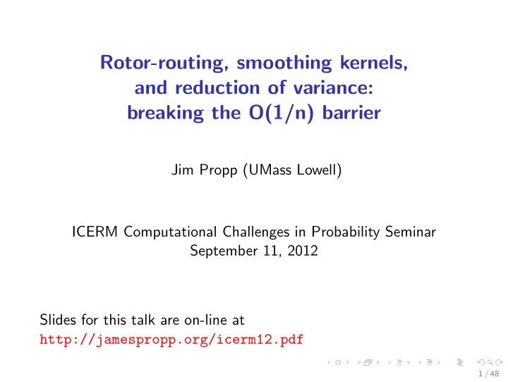
Rotor-routing, smoothing kernels, and reduction of variance: breaking the O(1/n) barrier Jim Propp (UMass Lowell) ICERM Computational Challenges in Probability Seminar September 11, 2012 Slides for this talk are on-line at http://jamespropp.org/icerm12.pdf 1 / 48

Acknowledgments This talk describes work that evolved from conversations and collaborations with David Einstein, Ander Holroyd, and Lionel Levine, as well as answers I received to questions I posted on MathOverflow (see http://mathoverflow.net ). 2 / 48

I. Introduction 3 / 48

Monte Carlo simulation (the two-minute course) Consider a sequence of identically distributed r.v.’s X 1 , X 2 , . . . with Law ( X n ) = Law ( X ) for all n . Let S n := X 1 + · · · + X n . Exp ( S n / n ) = Exp ( X ), and if the X n ’s are independent, the LLN says S n / n → Exp ( X ) almost surely. 4 / 48

Monte Carlo simulation (the two-minute course) When it’s easy to generate IID samples from Law ( X ) but hard to compute Exp ( X ), this gives a way to estimate Exp ( X ) empirically (the “Monte Carlo method’): Estimate Exp ( X ) by S n / n ∼ Exp ( X ) for some large n . If Var ( X ) is finite, then Var ( S n / n ) = Var ( S n ) / n 2 = n Var ( X ) / n 2 = Var ( X ) / n , so the standard deviation σ ( S n / n ) of our estimate is typically O (1 / √ n ). 5 / 48

Quasi-Monte Carlo, aka “Casablanca simulation” (Customer: “Are you sure this place is honest?”) Idea: We make σ ( S n / n ) smaller than O (1 / √ n ) by “cheating”, i.e., by using NON-independent, identically distributed r.v.’s. Here we are working in the space of all joinings Law ( X 1 , X 2 , . . . ) whose n th marginal is Law ( X ) for all n , and we are trying to simultaneously minimize the functionals Var ( S n / n ), or equivalently minimize the functionals Var ( S n ). Note that S n / n is automatically an unbiased estimator of Exp ( X ). 6 / 48

The Bernoulli case is special For most r.v.’s, these goals conflict. E.g., when Law ( X ) is uniform on [0 , 1], there are joinings for which Var ( S 2 ) is zero (easy), and other joinings for which Var ( S 3 ) is zero (a fun puzzle), but there’s no joining that achieves both at the same time. But when Law ( X ) is Bernoulli ( p ), there’s a law for X 1 , . . . , X n that simultaneously minimizes all of the Var ( S n )’s (with n ≥ 2). 7 / 48

The first “half” of this talk Such “maximally anticorrelated Bernoulli sequences” can be used as components of networks (“randomized rotor-router networks”) that compute anticorrelated sequences of r.v.’s of various kinds. I’ll apply this to a random variable associated with absorbing Markov chains (namely the indicator r.v. of absorption in a particular state) and show that with randomized rotor-routers we get Var ( S n / n ) = O (1 / n 2 ) (cf. Var ( S n / n ) = O (1 / n ) for IID). That is, the typical difference between S n / n and Exp ( X ) is O (1 / n ) rather than O (1 / √ n ). Moreover, I’ll show that the tail of the distribution of S n − Exp ( X ) isn’t just small; it vanishes beyond a certain point. 8 / 48

The second “half” of this talk The preceding result is clearly best possible; Var ( S n ) can’t be o (1), since S n − 1 and S n differ by an instance of X . So Var ( S n / n ) can’t be o (1 / n 2 ) and σ ( S n / n ) can’t be o (1 / n ). But in the last part of this talk, I’ll describe how to use X 1 , . . . , X n to get estimates of Exp ( X ) with typical error o (1 / n ). 9 / 48

II. Rotor-routing 10 / 48

“MAID” (Maximally Anticorrelated, Identically Distributed) Bernoulli sequences With 0 < p < 1, and U uniform in [0 , 1), let X n = ⌊ U + np ⌋ − ⌊ U + ( n − 1) p ⌋ ∈ { 0 , 1 } for all n ≥ 1. Then Law ( X n ) is Bernoulli ( p ), and S n = ⌊ U + np ⌋ − ⌊ U ⌋ ∈ {⌊ np ⌋ , ⌈ np ⌉} , so S n has variance as small as it can be, subject to Exp ( S n ) = np . ( X 1 , X 2 , . . . ) is a random Sturmian sequence of density p . 11 / 48

A physical model We have a spinner consisting of an arrow pinned to a disk; the center of the arrow is pinned to the center of a disk and the arrow is free to rotate. The disk has a black sector occupying a proportion 0 < p < 1 of the disk. If we were to repeatedly randomize the arrow, outputting a 1 or a 0 according to whether the arrow pointed into the black sector or not, we would get an IID Bernoulli ( p ) process. But instead we randomize the arrow just once at the start, and on subsequent turns we merely rotate it counterclockwise p turns around the circle, so that our sequence of 1’s and 0’s is a MAID Bernoulli ( p ) process. 12 / 48

Irrational p vs. rational p When p is irrational, there is a measure-preserving almost-bijection between the circle R / Z and the set of Sturmian sequences of density p . When p is rational, say p = a / b in lowest terms, then there are just b Sturmian sequences of density p , and the MAID Bernoulli ( p ) process gives them equal likelihood. E.g., for p = 2 / 5, the law of ( X 1 , X 2 , . . . ) is supported on five infinite sequences of period 5, each of which has probability 1/5: (1 , 0 , 1 , 0 , 0 , . . . ) (0 , 1 , 0 , 1 , 0 , . . . ) (0 , 0 , 1 , 0 , 1 , . . . ) (1 , 0 , 0 , 1 , 0 , . . . ) (0 , 1 , 0 , 0 , 1 , . . . ) 13 / 48

Markov chains and hitting probabilities Consider a finite-state absorbing Markov chain with a designated source-state s and absorbing states (“target-states”) t 1 , . . . , t m , such that Prob(the chain eventually enters { t 1 , . . . , t m } | the chain starts at state s ) = 1. Let t ∗ be one of the target states, and let p ∗ be the probability that the chain eventually enters state t ∗ . Then p ∗ = Exp ( X ), where X is 1 or 0 according to whether a run of the Markov chain leads to absorption at t ∗ or absorption elsewhere. 14 / 48

Particles on a directed graph It’s convenient to imagine that the states of the chain are vertices in a directed graph, and that the evolution of the chain corresponds to the trajectory of a particle that travels from the i th vertex to the j th vertex when the Markov chain goes from state i to state j . 15 / 48

Gambler’s ruin For simplicity, assume that each state i of the Markov chain has just two successors, with probabilities p i and 1 − p i . We’ll focus on the Markov chain with state-space { 0 , 1 , 2 , 3 } where 1 is the source and 0 and 3 are the targets, with all allowed transitions of the form i → i + 1 and i → i − 1, with Prob(1 → 2) = Prob(2 → 3) = p . (This corresponds to the purse-size of a gambler who starts out with $1 and makes a succession of bets, gaining $1 with probability p and losing $1 with probability 1 − p , until he either has $3 and leaves happy or has $0 and leaves broke.) Let t ∗ = 3. It’s easy to prove that p ∗ = p 2 / (1 − p + p 2 ). But what if we want to estimate p ∗ empirically by running the chain? 16 / 48

Monte Carlo made complicated To simulate the gambler’s ruin Markov chain repeatedly (in “supertime”) we use random variables U i , k ( i ∈ { 1 , 2 } , k ∈ { 1 , 2 , 3 , . . . } ) where U i , k is the source of randomness we use when, for the k th supertime, a run of the Markov chain has put us in state i . All the U i , k ’s are uniform in [0 , 1] and are independent of one another. If the chain is in non-absorbing state i at time t , let its state at time t + 1 be i + 1 if U i , k ∈ [0 , p i ) and i − 1 otherwise. 17 / 48

Monte Carlo made complicated 1 2 3 1 0 1 2 1 2 ... ... U 1 , 1 U 1 , 2 U 1 , 3 U 1 , 4 U 2 , 1 U 2 , 2 U 2 , 3 ... 18 / 48

Monte Carlo made complicated (It may be helpful to imagine a spinner at i that we spin each supertime the Markov chain is in state i .) When we reach a target state, we start again from the source state. Each run will result in absorption at 0 or absorption at 3, outputting a Bernoulli ( p ∗ ) bit. The successive Bernoulli ( p ∗ ) bits will be IID. 19 / 48

Anticorrelated quasi-Monte Carlo Instead of having each sequence U i , 1 , U i , 2 , . . . be IID, have each sequence be MAID. That is, U i , k +1 = U i , k + p i (mod 1). Once again there is a spinner at i , but instead of randomizing it each time we use it, we rotate it by p i turns (i.e., by an angle of 2 π p i ). We call this kind of spinner a rotor. 20 / 48

Rotor-routing (see Holroyd, Levine, M´ esz´ aros, Peres, P., and Wilson, “Chip-Firing and Rotor-Routing on Directed Graphs,” arXiv:0801.3306 ) The particle starts at i 1 = s . For t = 1 , 2 , . . . in succession, we update the rotor at i t (incrementing it by p i t (mod 1)) and use it to decide which i t +1 the particle should go to, until the particle gets absorbed at a target. Rotors can be used for general finite-state Markov chains (even when states have more than two successors), and indeed for some infinite-state Markov chains; see Holroyd and Propp, “Rotor Walks and Markov Chains”, arXiv:0904.4507 . 21 / 48

An example Consider $3 gambler’s ruin with p = 1 / 2. 1st particle: 1 → 0 2nd particle: 1 → 2 → 3 3rd particle: 1 → 0 4th particle: 1 → 2 → 1 → 0 5th particle: 1 → 2 → 3 6th particle: 1 → 0 7th particle: 1 → 2 → 1 → 0 etc. (with period 3) 22 / 48

“Let’s see that again in configuration space” i = 1 i = 2 → ← ⇓ absorption at 0 ← ← ⇓ absorption at 3 → → ⇓ absorption at 0 ← → ⇓ absorption at 0 ← ← ⇓ absorption at 3 → → ⇓ absorption at 0 ← → ⇓ . . . 23 / 48