Overview: Kernels for Sequences and Graphs String Kernels 8 - PowerPoint PPT Presentation
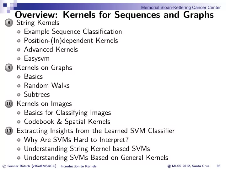
Memorial Sloan-Kettering Cancer Center Overview: Kernels for Sequences and Graphs String Kernels 8 Example Sequence Classification Position-(In)dependent Kernels Advanced Kernels Easysvm Kernels on Graphs 9 Basics Random Walks Subtrees
Memorial Sloan-Kettering Cancer Center Regulatory Modules Kernel [Schultheiss et al., 2008] Search for overrepresented motifs m 1 , . . . , m M (colored bars) Find best match of motif m i in example x j ; extract windows s i , j at position p i , j around matches (boxed) Use a string kernel, e.g. k WDS , on all extracted sequence windows, and define a combined kernel for the sequences: k seq ( x j , x k ) = � M i =1 k WDS ( s i , j , s i , k ) Use a second kernel k pos , e.g. based on RBF kernel, on vector of pairwise distances between the motif matches: f j = ( p 1 , j − p 2 , j , p 1 , j − p 3 , j , . . . , p M − 1 , j − p M , j ) Regulatory Modules kernel: k RM ( x , x ′ ) := k seq ( x , x ′ ) + k pos ( x , x ′ ) @ MLSS 2012, Santa Cruz � Gunnar R¨ c atsch ( cBio@MSKCC ) Introduction to Kernels 106
Memorial Sloan-Kettering Cancer Center Regulatory Modules Kernel [Schultheiss et al., 2008] Search for overrepresented motifs m 1 , . . . , m M (colored bars) Find best match of motif m i in example x j ; extract windows s i , j at position p i , j around matches (boxed) Use a string kernel, e.g. k WDS , on all extracted sequence windows, and define a combined kernel for the sequences: k seq ( x j , x k ) = � M i =1 k WDS ( s i , j , s i , k ) Use a second kernel k pos , e.g. based on RBF kernel, on vector of pairwise distances between the motif matches: f j = ( p 1 , j − p 2 , j , p 1 , j − p 3 , j , . . . , p M − 1 , j − p M , j ) Regulatory Modules kernel: k RM ( x , x ′ ) := k seq ( x , x ′ ) + k pos ( x , x ′ ) @ MLSS 2012, Santa Cruz � Gunnar R¨ c atsch ( cBio@MSKCC ) Introduction to Kernels 106
Memorial Sloan-Kettering Cancer Center Regulatory Modules Kernel [Schultheiss et al., 2008] Search for overrepresented motifs m 1 , . . . , m M (colored bars) Find best match of motif m i in example x j ; extract windows s i , j at position p i , j around matches (boxed) Use a string kernel, e.g. k WDS , on all extracted sequence windows, and define a combined kernel for the sequences: k seq ( x j , x k ) = � M i =1 k WDS ( s i , j , s i , k ) Use a second kernel k pos , e.g. based on RBF kernel, on vector of pairwise distances between the motif matches: f j = ( p 1 , j − p 2 , j , p 1 , j − p 3 , j , . . . , p M − 1 , j − p M , j ) Regulatory Modules kernel: k RM ( x , x ′ ) := k seq ( x , x ′ ) + k pos ( x , x ′ ) @ MLSS 2012, Santa Cruz � Gunnar R¨ c atsch ( cBio@MSKCC ) Introduction to Kernels 106
Memorial Sloan-Kettering Cancer Center Regulatory Modules Kernel [Schultheiss et al., 2008] Search for overrepresented motifs m 1 , . . . , m M (colored bars) Find best match of motif m i in example x j ; extract windows s i , j at position p i , j around matches (boxed) Use a string kernel, e.g. k WDS , on all extracted sequence windows, and define a combined kernel for the sequences: k seq ( x j , x k ) = � M i =1 k WDS ( s i , j , s i , k ) Use a second kernel k pos , e.g. based on RBF kernel, on vector of pairwise distances between the motif matches: f j = ( p 1 , j − p 2 , j , p 1 , j − p 3 , j , . . . , p M − 1 , j − p M , j ) Regulatory Modules kernel: k RM ( x , x ′ ) := k seq ( x , x ′ ) + k pos ( x , x ′ ) @ MLSS 2012, Santa Cruz � Gunnar R¨ c atsch ( cBio@MSKCC ) Introduction to Kernels 106
Memorial Sloan-Kettering Cancer Center Local Alignment Kernel In order to compute the score of an alignment, one needs: gap penalty substitution matrix S ∈ R Σ × Σ g : N → R An alignment π is then scored as follows: CGGSLIAMM----WFGV |...|||||....|||| C---LIVMMNRLMWFGV s S , g ( π ) = S ( C , C ) + S ( L , L ) + S ( I , I ) + S ( A , V ) + 2 S ( M , M ) + S ( W , W ) + S ( F , F ) + S ( G , G ) + S ( V , V ) − g (3) − g (4) Smith-Waterman score (not positive definite) SW S , g ( x , y ) := max π ∈ Π( x , y ) s S , g ( π ) Local Alignment kernel [Vert et al., 2004] K β ( x , y ) = � π ∈ Π( x , y ) exp( β s S , g ( π )) @ MLSS 2012, Santa Cruz � Gunnar R¨ c atsch ( cBio@MSKCC ) Introduction to Kernels 107
Memorial Sloan-Kettering Cancer Center Local Alignment Kernel In order to compute the score of an alignment, one needs: gap penalty substitution matrix S ∈ R Σ × Σ g : N → R An alignment π is then scored as follows: CGGSLIAMM----WFGV |...|||||....|||| C---LIVMMNRLMWFGV s S , g ( π ) = S ( C , C ) + S ( L , L ) + S ( I , I ) + S ( A , V ) + 2 S ( M , M ) + S ( W , W ) + S ( F , F ) + S ( G , G ) + S ( V , V ) − g (3) − g (4) Smith-Waterman score (not positive definite) SW S , g ( x , y ) := max π ∈ Π( x , y ) s S , g ( π ) Local Alignment kernel [Vert et al., 2004] K β ( x , y ) = � π ∈ Π( x , y ) exp( β s S , g ( π )) @ MLSS 2012, Santa Cruz � Gunnar R¨ c atsch ( cBio@MSKCC ) Introduction to Kernels 107
Memorial Sloan-Kettering Cancer Center Local Alignment Kernel In order to compute the score of an alignment, one needs: gap penalty substitution matrix S ∈ R Σ × Σ g : N → R An alignment π is then scored as follows: CGGSLIAMM----WFGV |...|||||....|||| C---LIVMMNRLMWFGV s S , g ( π ) = S ( C , C ) + S ( L , L ) + S ( I , I ) + S ( A , V ) + 2 S ( M , M ) + S ( W , W ) + S ( F , F ) + S ( G , G ) + S ( V , V ) − g (3) − g (4) Smith-Waterman score (not positive definite) SW S , g ( x , y ) := max π ∈ Π( x , y ) s S , g ( π ) Local Alignment kernel [Vert et al., 2004] K β ( x , y ) = � π ∈ Π( x , y ) exp( β s S , g ( π )) @ MLSS 2012, Santa Cruz � Gunnar R¨ c atsch ( cBio@MSKCC ) Introduction to Kernels 107
Memorial Sloan-Kettering Cancer Center Locality-Improved Kernel Polynomial Kernel of degree d : Σ �� l � d k POLY ( x , x ′ ) = p =1 I p ( x , x ′ ) ⇒ Computes all d -th order monomials: global information A C d . (. .) G A T T d . Locality-Improved Kernel [Zien et al., 2000] (. .) C G T A d . � N (. .) T T k LI ( x , y ) = p =1 win p ( x , y ) G T d . C (. .) A A A �� + l � d d . (. .) A G win p ( x , y ) = j = − l p j I p + j ( x , y ) Sequence Sequence x x’ � x i = x ′ local/global information 1 , I i ( x , x ′ ) = i 0 , otherwise @ MLSS 2012, Santa Cruz � Gunnar R¨ c atsch ( cBio@MSKCC ) Introduction to Kernels 108
Memorial Sloan-Kettering Cancer Center Fisher & TOP Kernel General idea [Jaakkola et al., 2000; Tsuda et al., 2002a] Combine probabilistic models and SVMs Sequence representation Sequences s of arbitrary length Probabilistic model p ( s | θ ) (e.g. HMM, PSSMs) Maximum likelihood estimate θ ∗ ∈ R d Transformation into Fisher score features Φ( s ) ∈ R d Φ( s ) = ∂ log( p ( s | θ )) ∂ θ Describes contribution of every parameter to p ( s | θ ) k ( s , s ′ ) = � Φ( s ) , Φ( s ′ ) � @ MLSS 2012, Santa Cruz � Gunnar R¨ c atsch ( cBio@MSKCC ) Introduction to Kernels 109
Memorial Sloan-Kettering Cancer Center Example: Fisher Kernel on PSSMs Sequences s ∈ Σ N of fixed length PSSMs: log p ( s | θ ) = log � N i =1 θ i , s i = � N i =1 log θ i , s i =: � N i =1 θ log i , s i Fisher score features: (Φ( s )) i ,σ = d p ( s | θ log ) = Id ( s i = σ ) d θ log i ,σ N � Kernel: k ( s , s ′ ) = � Φ( s ) , Φ( s ′ ) � = Id ( s i = s ′ i ) i =1 Identical to WD kernel with order 1 Note: Marginalized-count kernels [Tsuda et al., 2002b] can be understood as a generalization of Fisher kernels. See e.g. [Sonnenburg, 2002] @ MLSS 2012, Santa Cruz � Gunnar R¨ c atsch ( cBio@MSKCC ) Introduction to Kernels 110
Memorial Sloan-Kettering Cancer Center Pairwise Comparison Kernels General idea [Liao and Noble, 2002] Employ empirical kernel map on Smith-Waterman/BLAST scores Advantage Utilizes decades of practical experience with BLAST High computational cost ( O ( N 3 )) Disadvantage Alleviation Employ Blast instead of Smith-Waterman Use a smaller subset for empirical map @ MLSS 2012, Santa Cruz � Gunnar R¨ c atsch ( cBio@MSKCC ) Introduction to Kernels 111
Memorial Sloan-Kettering Cancer Center Summary of String Kernels Kernel l x � = l x ′ Pr ( x | θ ) Posi- Scope Com- tional? plexity linear no no yes local O ( l x ) polynomial no no yes global O ( l x ) locality-improved no no yes local/global O ( l · l x ) sub-sequence yes no yes global O ( nl x l x ′ ) O ( l x ) n-gram/Spectrum yes no no global O ( l x ) WD no no yes local local/global O ( s · l x ) WD with shifts no no yes local/global O ( l x l x ′ ) Oligo yes no yes TOP yes/no yes yes/no local/global depends Fisher yes/no yes yes/no local/global depends @ MLSS 2012, Santa Cruz � Gunnar R¨ c atsch ( cBio@MSKCC ) Introduction to Kernels 112
Memorial Sloan-Kettering Cancer Center Live Demonstration Please check out instructions at http://raetschlab.org/lectures/ MLSSKernelTutorial2012/demo @ MLSS 2012, Santa Cruz � Gunnar R¨ c atsch ( cBio@MSKCC ) Introduction to Kernels 113
Memorial Sloan-Kettering Cancer Center Illustration Using Galaxy Web Service Task 1: Learn to classify acceptor splice sites with GC features 1 Train classifier and predict using 5-fold cross-validation ( SVM Toolbox → Train and Test SVM ) 2 Evaluate classifier ( SVM Toolbox → Evaluate Predictions ) Steps: 1 Use “ Upload file ” with URL http://svmcompbio.tuebingen. mpg.de/data/C_elegans_acc_gc.arff ; set file format to ARFF and upload; file appears in history on right 2 Use “ Train and Test SVM ” on uploaded data set (choose ARFF data format) tool; set the kernel to linear , execute and look at the result 3 Use “ Evaluate Predictions ” on predictions and the labeled data (choose ARFF format), select ROC Curve and execute; check out the evaluation summary and the ROC curves @ MLSS 2012, Santa Cruz � Gunnar R¨ c atsch ( cBio@MSKCC ) Introduction to Kernels 114
Memorial Sloan-Kettering Cancer Center Illustration Using Galaxy Web Service Task 1: Learn to classify acceptor splice sites with GC features 1 Train classifier and predict using 5-fold cross-validation ( SVM Toolbox → Train and Test SVM ) 2 Evaluate classifier ( SVM Toolbox → Evaluate Predictions ) Steps: 1 Use “ Upload file ” with URL http://svmcompbio.tuebingen. mpg.de/data/C_elegans_acc_gc.arff ; set file format to ARFF and upload; file appears in history on right 2 Use “ Train and Test SVM ” on uploaded data set (choose ARFF data format) tool; set the kernel to linear , execute and look at the result 3 Use “ Evaluate Predictions ” on predictions and the labeled data (choose ARFF format), select ROC Curve and execute; check out the evaluation summary and the ROC curves @ MLSS 2012, Santa Cruz � Gunnar R¨ c atsch ( cBio@MSKCC ) Introduction to Kernels 114
Memorial Sloan-Kettering Cancer Center Illustration Using Galaxy Web Service Task 1: Learn to classify acceptor splice sites with GC features 1 Train classifier and predict using 5-fold cross-validation ( SVM Toolbox → Train and Test SVM ) 2 Evaluate classifier ( SVM Toolbox → Evaluate Predictions ) Steps: 1 Use “ Upload file ” with URL http://svmcompbio.tuebingen. mpg.de/data/C_elegans_acc_gc.arff ; set file format to ARFF and upload; file appears in history on right 2 Use “ Train and Test SVM ” on uploaded data set (choose ARFF data format) tool; set the kernel to linear , execute and look at the result 3 Use “ Evaluate Predictions ” on predictions and the labeled data (choose ARFF format), select ROC Curve and execute; check out the evaluation summary and the ROC curves @ MLSS 2012, Santa Cruz � Gunnar R¨ c atsch ( cBio@MSKCC ) Introduction to Kernels 114
Memorial Sloan-Kettering Cancer Center Illustration Using Galaxy Web Service Task 1: Learn to classify acceptor splice sites with GC features 1 Train classifier and predict using 5-fold cross-validation ( SVM Toolbox → Train and Test SVM ) 2 Evaluate classifier ( SVM Toolbox → Evaluate Predictions ) Steps: 1 Use “ Upload file ” with URL http://svmcompbio.tuebingen. mpg.de/data/C_elegans_acc_gc.arff ; set file format to ARFF and upload; file appears in history on right 2 Use “ Train and Test SVM ” on uploaded data set (choose ARFF data format) tool; set the kernel to linear , execute and look at the result 3 Use “ Evaluate Predictions ” on predictions and the labeled data (choose ARFF format), select ROC Curve and execute; check out the evaluation summary and the ROC curves @ MLSS 2012, Santa Cruz � Gunnar R¨ c atsch ( cBio@MSKCC ) Introduction to Kernels 114
Memorial Sloan-Kettering Cancer Center Demonstration Using Galaxy Webservice Task 1: Learn to classify acceptor splice sites with sequences 1 Train classifier and predict, using 5-fold cross-validation ( SVM Toolbox → Train and Test SVM ) 2 Evaluate classifier ( SVM Toolbox → Evaluate Predictions ) Steps: 1 Use “ Upload file ” with URL http://svmcompbio.tuebingen. mpg.de/data/C_elegans_acc_seq.arff . Set file format to ARFF and upload. 2 Use “ Train and Test SVM ” on uploaded dataset (choose ARFF data format) tool. Set the kernel to a) Spectrum with degree=6 and b) Weight Degree with degree=6 and shift=0. Execute and look at the result. 3 Use “ Evaluate Predictions ” on predictions and the labeled data (choose ARFF format). Select ROC Curve and execute. Check out the evaluation summary and the ROC curves. @ MLSS 2012, Santa Cruz � Gunnar R¨ c atsch ( cBio@MSKCC ) Introduction to Kernels 115
Memorial Sloan-Kettering Cancer Center Demonstration Using Galaxy Webservice Task 1: Learn to classify acceptor splice sites with sequences 1 Train classifier and predict, using 5-fold cross-validation ( SVM Toolbox → Train and Test SVM ) 2 Evaluate classifier ( SVM Toolbox → Evaluate Predictions ) Steps: 1 Use “ Upload file ” with URL http://svmcompbio.tuebingen. mpg.de/data/C_elegans_acc_seq.arff . Set file format to ARFF and upload. 2 Use “ Train and Test SVM ” on uploaded dataset (choose ARFF data format) tool. Set the kernel to a) Spectrum with degree=6 and b) Weight Degree with degree=6 and shift=0. Execute and look at the result. 3 Use “ Evaluate Predictions ” on predictions and the labeled data (choose ARFF format). Select ROC Curve and execute. Check out the evaluation summary and the ROC curves. @ MLSS 2012, Santa Cruz � Gunnar R¨ c atsch ( cBio@MSKCC ) Introduction to Kernels 115
Memorial Sloan-Kettering Cancer Center Demonstration Using Galaxy Webservice Task 1: Learn to classify acceptor splice sites with sequences 1 Train classifier and predict, using 5-fold cross-validation ( SVM Toolbox → Train and Test SVM ) 2 Evaluate classifier ( SVM Toolbox → Evaluate Predictions ) Steps: 1 Use “ Upload file ” with URL http://svmcompbio.tuebingen. mpg.de/data/C_elegans_acc_seq.arff . Set file format to ARFF and upload. 2 Use “ Train and Test SVM ” on uploaded dataset (choose ARFF data format) tool. Set the kernel to a) Spectrum with degree=6 and b) Weight Degree with degree=6 and shift=0. Execute and look at the result. 3 Use “ Evaluate Predictions ” on predictions and the labeled data (choose ARFF format). Select ROC Curve and execute. Check out the evaluation summary and the ROC curves. @ MLSS 2012, Santa Cruz � Gunnar R¨ c atsch ( cBio@MSKCC ) Introduction to Kernels 115
Memorial Sloan-Kettering Cancer Center Demonstration Using Galaxy Webservice Task 1: Learn to classify acceptor splice sites with sequences 1 Train classifier and predict, using 5-fold cross-validation ( SVM Toolbox → Train and Test SVM ) 2 Evaluate classifier ( SVM Toolbox → Evaluate Predictions ) Steps: 1 Use “ Upload file ” with URL http://svmcompbio.tuebingen. mpg.de/data/C_elegans_acc_seq.arff . Set file format to ARFF and upload. 2 Use “ Train and Test SVM ” on uploaded dataset (choose ARFF data format) tool. Set the kernel to a) Spectrum with degree=6 and b) Weight Degree with degree=6 and shift=0. Execute and look at the result. 3 Use “ Evaluate Predictions ” on predictions and the labeled data (choose ARFF format). Select ROC Curve and execute. Check out the evaluation summary and the ROC curves. @ MLSS 2012, Santa Cruz � Gunnar R¨ c atsch ( cBio@MSKCC ) Introduction to Kernels 115
Memorial Sloan-Kettering Cancer Center Illustration Using Galaxy Web Service Task 2: Determine the best combination of polynomial degree d = 1 , . . . , 5 and SVMs C = { 0 . 1 , 1 , 10 } using 5-fold cross-validation ( SVM Toolbox → SVM Model Selection ) Steps: 1 Reuse the uploaded file from Task 1. 2 Use “ SVM Model Selection ” with uploaded data (choose ARFF format), set the number of cross-validation rounds to 5, set C ’s as 0 . 1 , 1 , 10, select the polynomial kernel and choose the degrees as 1 , 2 , 3 , 4 , 5. Execute and check the results. @ MLSS 2012, Santa Cruz � Gunnar R¨ c atsch ( cBio@MSKCC ) Introduction to Kernels 116
Memorial Sloan-Kettering Cancer Center Illustration Using Galaxy Web Service Task 2: Determine the best combination of polynomial degree d = 1 , . . . , 5 and SVMs C = { 0 . 1 , 1 , 10 } using 5-fold cross-validation ( SVM Toolbox → SVM Model Selection ) Steps: 1 Reuse the uploaded file from Task 1. 2 Use “ SVM Model Selection ” with uploaded data (choose ARFF format), set the number of cross-validation rounds to 5, set C ’s as 0 . 1 , 1 , 10, select the polynomial kernel and choose the degrees as 1 , 2 , 3 , 4 , 5. Execute and check the results. @ MLSS 2012, Santa Cruz � Gunnar R¨ c atsch ( cBio@MSKCC ) Introduction to Kernels 116
Memorial Sloan-Kettering Cancer Center Illustration Using Galaxy Web Service Task 2: Determine the best combination of polynomial degree d = 1 , . . . , 5 and SVMs C = { 0 . 1 , 1 , 10 } using 5-fold cross-validation ( SVM Toolbox → SVM Model Selection ) Steps: 1 Reuse the uploaded file from Task 1. 2 Use “ SVM Model Selection ” with uploaded data (choose ARFF format), set the number of cross-validation rounds to 5, set C ’s as 0 . 1 , 1 , 10, select the polynomial kernel and choose the degrees as 1 , 2 , 3 , 4 , 5. Execute and check the results. @ MLSS 2012, Santa Cruz � Gunnar R¨ c atsch ( cBio@MSKCC ) Introduction to Kernels 116
Memorial Sloan-Kettering Cancer Center Do-it-yourself with Easysvm (Prep) Install Shogun toolbox: wget http://shogun-toolbox.org/archives/shogun/releases/0.7/sources/shogun-0.7.3.tar.bz2 tar xjf shogun-0.7.3.tar.bz2 cd shogun-0.7.3/src ./configure --interfaces=python_modular,libshogun,libshogunui --prefix=~/mylibs make && make install && cd ../.. export PYTHONPATH=~/mylibs/lib/python2.?/site-packages; export LD_LIBRARY_PATH=~/mylibs/lib; export DYLD_LIBRARY_PATH=$LD_LIBRARY_PATH Install Easysvm and get data: wget http://www.fml.tuebingen.mpg.de/raetsch/projects/easysvm/easysvm-0.3.1.tar.gz tar xzf easysvm-0.3.1.tar.gz cd easysvm-0.3.1 && python setup.py install --prefix=~/mylibs && cd .. wget http://svmcompbio.tuebingen.mpg.de/data/C_elegans_acc_gc.arff wget http://svmcompbio.tuebingen.mpg.de/data/C_elegans_acc_seq.arff @ MLSS 2012, Santa Cruz � Gunnar R¨ c atsch ( cBio@MSKCC ) Introduction to Kernels 117
Memorial Sloan-Kettering Cancer Center Do-it-yourself with Easysvm Task 1: Learn to classify acceptor splice sites with GC features 1 Train classifier and predict using 5-fold cross-validation ( cv ) 2 Evaluate classifier ( eval ) SVM C predictions kernel data format and file ���� � �� � � �� � � �� � ~/mylibs/bin/easysvm.py cv 5 1 linear arff C_elegans_acc_gc.arff lin_gc.out 2 features, 2200 examples Using 5-fold crossvalidation head -4 lin_gc.out #example output split 0 -0.8740213 0 1 -0.9755172 2 2 -0.9060478 1 predictions output file data format and file � �� � � �� � � �� � ~/mylibs/bin/easysvm.py eval lin_gc.out arff C_elegans_acc_gc.arff lin_gc.perf tail -6 lin_gc.perf Averages Number of positive examples = 40 Number of negative examples = 400 Area under ROC curve = 91.3 % Area under PRC curve = 55.8 % Accuracy (at threshold 0) = 90.9 % @ MLSS 2012, Santa Cruz � Gunnar R¨ c atsch ( cBio@MSKCC ) Introduction to Kernels 118
Memorial Sloan-Kettering Cancer Center Do-it-yourself with Easysvm Task 2: Determine the best combination of polynomial degree d = 1 , . . . , 5 and SVMs C = { 0 . 1 , 1 , 10 } using 5-fold cross-validation (modelsel) kernel & parameters SVM C ’s � �� � � �� � ~/mylibs/bin/easysvm.py modelsel 5 0 . 1 , 1 , 10 poly 1,2,3,4,5 true false \ output file data format and file � �� � � �� � arff C_elegans_acc_gc.arff poly_gc.modelsel 2 features, 2200 examples Using 5-fold crossvalidation ... head -8 poly_gc.modelsel Best model(s) according to ROC measure: C=10.0 degree=1 Best model(s) according to PRC measure: C=1.0 degree=1 Best model(s) according to accuracy measure: C=10.0 degree=1 ... @ MLSS 2012, Santa Cruz � Gunnar R¨ c atsch ( cBio@MSKCC ) Introduction to Kernels 119
Memorial Sloan-Kettering Cancer Center Demonstration with Easysvm Task 1: Learn to classify acceptor splice sites with sequences 1 Train classifier and predict using 5-fold cross-validation ( cv ) 2 Evaluate classifier ( eval ) SVM C predictions kernel data format and file ���� � �� � � �� � � �� � ~/mylibs/bin/easysvm.py cv 5 1 spec 6 arff C_elegans_acc_seq.arff spec_seq.out predictions output file data format and file � �� � � �� � � �� � ~/mylibs/bin/easysvm.py eval spec_seq.out arff C_elegans_acc_seq.arff spec_seq.perf tail -3 spec_seq.perf Area under ROC curve = 80.4 % Area under PRC curve = 33.7 % accuracy (at threshold 0) = 90.8 % SVM C predictions kernel data format and file ���� � �� � � �� � � �� � ~/mylibs/bin/easysvm.py cv 5 1 WD 6 0 arff C_elegans_acc_seq.arff wd_seq.out predictions output file data format and file � �� � � �� � � �� � ~/mylibs/bin/easysvm.py eval wd_seq.out arff C_elegans_acc_gc.arff wd_seq.perf tail -6 wd_seq.perf Area under ROC curve = 98.8 % Area under PRC curve = 87.5 % Accuracy (at threshold 0) = 97.0 % @ MLSS 2012, Santa Cruz � Gunnar R¨ c atsch ( cBio@MSKCC ) Introduction to Kernels 120
Memorial Sloan-Kettering Cancer Center Kernels on Graphs Graphs are everywhere . . . Graphs in Reality Graphs model objects and their relationships. Also referred to as networks . All common data structures can be modelled as graphs. Graphs in Bioinformatics Molecular biology studies relationships between molecular components. Graphs are ideal to model: Molecules Protein-protein interaction networks Metabolic networks @ MLSS 2012, Santa Cruz � Gunnar R¨ c atsch ( cBio@MSKCC ) Introduction to Kernels 121
Memorial Sloan-Kettering Cancer Center Kernels on Graphs Graphs are everywhere . . . Graphs in Reality Graphs model objects and their relationships. Also referred to as networks . All common data structures can be modelled as graphs. Graphs in Bioinformatics Molecular biology studies relationships between molecular components. Graphs are ideal to model: Molecules Protein-protein interaction networks Metabolic networks @ MLSS 2012, Santa Cruz � Gunnar R¨ c atsch ( cBio@MSKCC ) Introduction to Kernels 121
Memorial Sloan-Kettering Cancer Center Central Questions How similar are two graphs? Graph similarity is the central problem for all learning tasks such as clustering and classification on graphs. Applications Function prediction for molecules, in particular, proteins Comparison of protein-protein interaction networks Challenges Subgraph isomorphism is NP-complete. Comparing graphs via isomorphism checking is thus prohibitively expensive! Graph kernels offer a faster, yet one based on sound principles. @ MLSS 2012, Santa Cruz � Gunnar R¨ c atsch ( cBio@MSKCC ) Introduction to Kernels 122
Memorial Sloan-Kettering Cancer Center Central Questions How similar are two graphs? Graph similarity is the central problem for all learning tasks such as clustering and classification on graphs. Applications Function prediction for molecules, in particular, proteins Comparison of protein-protein interaction networks Challenges Subgraph isomorphism is NP-complete. Comparing graphs via isomorphism checking is thus prohibitively expensive! Graph kernels offer a faster, yet one based on sound principles. @ MLSS 2012, Santa Cruz � Gunnar R¨ c atsch ( cBio@MSKCC ) Introduction to Kernels 122
Memorial Sloan-Kettering Cancer Center Central Questions How similar are two graphs? Graph similarity is the central problem for all learning tasks such as clustering and classification on graphs. Applications Function prediction for molecules, in particular, proteins Comparison of protein-protein interaction networks Challenges Subgraph isomorphism is NP-complete. Comparing graphs via isomorphism checking is thus prohibitively expensive! Graph kernels offer a faster, yet one based on sound principles. @ MLSS 2012, Santa Cruz � Gunnar R¨ c atsch ( cBio@MSKCC ) Introduction to Kernels 122
Memorial Sloan-Kettering Cancer Center From the beginning . . . Definition of a Graph A graph G is a set of nodes (or vertices) V and edges E , where E ⊂ V 2 . An attributed graph is a graph with labels on nodes and/or edges; we refer to labels as attributes . The adjacency matrix A of G is defined as � 1 if ( v i , v j ) ∈ E , [ A ] ij = otherwise , 0 where v i and v j are nodes in G . A walk w of length k − 1 in a graph is a sequence of nodes w = ( v 1 , v 2 , · · · , v k ) where ( v i − 1 , v i ) ∈ E for 1 ≤ i ≤ k . w is a path if v i � = v j for i � = j . @ MLSS 2012, Santa Cruz � Gunnar R¨ c atsch ( cBio@MSKCC ) Introduction to Kernels 123
Memorial Sloan-Kettering Cancer Center From the beginning . . . Definition of a Graph A graph G is a set of nodes (or vertices) V and edges E , where E ⊂ V 2 . An attributed graph is a graph with labels on nodes and/or edges; we refer to labels as attributes . The adjacency matrix A of G is defined as � 1 if ( v i , v j ) ∈ E , [ A ] ij = otherwise , 0 where v i and v j are nodes in G . A walk w of length k − 1 in a graph is a sequence of nodes w = ( v 1 , v 2 , · · · , v k ) where ( v i − 1 , v i ) ∈ E for 1 ≤ i ≤ k . w is a path if v i � = v j for i � = j . @ MLSS 2012, Santa Cruz � Gunnar R¨ c atsch ( cBio@MSKCC ) Introduction to Kernels 123
Memorial Sloan-Kettering Cancer Center From the beginning . . . Definition of a Graph A graph G is a set of nodes (or vertices) V and edges E , where E ⊂ V 2 . An attributed graph is a graph with labels on nodes and/or edges; we refer to labels as attributes . The adjacency matrix A of G is defined as � 1 if ( v i , v j ) ∈ E , [ A ] ij = otherwise , 0 where v i and v j are nodes in G . A walk w of length k − 1 in a graph is a sequence of nodes w = ( v 1 , v 2 , · · · , v k ) where ( v i − 1 , v i ) ∈ E for 1 ≤ i ≤ k . w is a path if v i � = v j for i � = j . @ MLSS 2012, Santa Cruz � Gunnar R¨ c atsch ( cBio@MSKCC ) Introduction to Kernels 123
Memorial Sloan-Kettering Cancer Center Graph Isomorphism Graph isomorphism (cf. Skiena, 1998) Find a mapping f of the vertices of G to the vertices of H such that G and H are identical; i.e. ( x , y ) is an edge of G iff ( f ( x ) , f ( y )) is an edge of H. Then f is an isomorphism, and G and F are called isomorphic. No polynomial-time algorithm is known for graph isomorphism Neither is it known to be NP-complete Subgraph isomorphism Subgraph isomorpism asks if there is a subset of edges and vertices of G that is isomorphic to a smaller graph H. Subgraph isomorphism is NP-complete @ MLSS 2012, Santa Cruz � Gunnar R¨ c atsch ( cBio@MSKCC ) Introduction to Kernels 124
Memorial Sloan-Kettering Cancer Center Graph Isomorphism Graph isomorphism (cf. Skiena, 1998) Find a mapping f of the vertices of G to the vertices of H such that G and H are identical; i.e. ( x , y ) is an edge of G iff ( f ( x ) , f ( y )) is an edge of H. Then f is an isomorphism, and G and F are called isomorphic. No polynomial-time algorithm is known for graph isomorphism Neither is it known to be NP-complete Subgraph isomorphism Subgraph isomorpism asks if there is a subset of edges and vertices of G that is isomorphic to a smaller graph H. Subgraph isomorphism is NP-complete @ MLSS 2012, Santa Cruz � Gunnar R¨ c atsch ( cBio@MSKCC ) Introduction to Kernels 124
Memorial Sloan-Kettering Cancer Center Polynomial Alternatives Graph kernels Compare substructures of graphs that are computable in polynomial time Examples: walks, paths, cyclic patterns, trees Criteria for a good graph kernel Expressive Efficient to compute Positive definite Applicable to wide range of graphs @ MLSS 2012, Santa Cruz � Gunnar R¨ c atsch ( cBio@MSKCC ) Introduction to Kernels 125
Memorial Sloan-Kettering Cancer Center Polynomial Alternatives Graph kernels Compare substructures of graphs that are computable in polynomial time Examples: walks, paths, cyclic patterns, trees Criteria for a good graph kernel Expressive Efficient to compute Positive definite Applicable to wide range of graphs @ MLSS 2012, Santa Cruz � Gunnar R¨ c atsch ( cBio@MSKCC ) Introduction to Kernels 125
Memorial Sloan-Kettering Cancer Center Random Walks Principle Compare walks in two input graphs Walks are sequences of nodes that allow repetitions of nodes Important trick Walks of length k can be computed by taking the adjacency matrix A to the power of k A k ( i , j ) = c means that c walks of length k exist between vertex i and vertex j @ MLSS 2012, Santa Cruz � Gunnar R¨ c atsch ( cBio@MSKCC ) Introduction to Kernels 126
Memorial Sloan-Kettering Cancer Center Product Graph How to find common walks in two graphs? Use the product graph of G 1 and G 2 Definition G × = ( V × , E × ), defined via V × ( G 1 × G 2 ) = { ( v 1 , w 1 ) ∈ V 1 × V 2 : label ( v 1 ) = label ( w 1 ) } { (( v 1 , w 1 ) , ( v 2 , w 2 )) ∈ V 2 ( G 1 × G 2 ) E × ( G 1 × G 2 ) = ( v 1 , v 2 ) ∈ E 1 ∧ ( w 1 , w 2 ) ∈ E 2 ∧ ( label ( v 1 , v 2 ) = label ( w 1 , w 2 )) } Meaning Product graph consists of pairs of identically labeled nodes and edges from G 1 and G 2 @ MLSS 2012, Santa Cruz � Gunnar R¨ c atsch ( cBio@MSKCC ) Introduction to Kernels 127
Memorial Sloan-Kettering Cancer Center Random Walk Kernel The trick Common walks can now be computed from A k × Definition of random walk kernel | V × | ∞ � � λ n A n k × ( G 1 , G 2 ) = [ × ] ij , i , j =1 n =0 Meaning Random walk kernel counts all pairs of matching walks λ is decaying factor for the sum to converge @ MLSS 2012, Santa Cruz � Gunnar R¨ c atsch ( cBio@MSKCC ) Introduction to Kernels 128
Memorial Sloan-Kettering Cancer Center Runtime of Random Walk Kernels Notation given two graphs G 1 and G 2 n is the number of nodes in G 1 and G 2 Computing product graph requires comparison of all pairs of edges in G 1 and G 2 runtime O ( n 4 ) Powers of adjacency matrix matrix multiplication or inversion for n 2 * n 2 matrix runtime O ( n 6 ) Total runtime O ( n 6 ) @ MLSS 2012, Santa Cruz � Gunnar R¨ c atsch ( cBio@MSKCC ) Introduction to Kernels 129
Memorial Sloan-Kettering Cancer Center Tottering Artificially high similarity scores Walk kernels allow walks to visit same edges and nodes multiple times → artificially high similarity scores by repeated visits to same two nodes Additional node labels Mah´ e et al. [2004] add additional node labels to reduce number of matching nodes → improved classification accuracy Forbidding cycles with 2 nodes Mah´ e et al. [2004] redefine walk kernel to forbid subcycles consisting of two nodes → no practical improvement @ MLSS 2012, Santa Cruz � Gunnar R¨ c atsch ( cBio@MSKCC ) Introduction to Kernels 130
Memorial Sloan-Kettering Cancer Center Limitations of Walks Different graphs mapped to identical points in walks feature space [Ramon and G¨ artner, 2003] @ MLSS 2012, Santa Cruz � Gunnar R¨ c atsch ( cBio@MSKCC ) Introduction to Kernels 131
Memorial Sloan-Kettering Cancer Center Subtree Kernel (Idea only) Motivation Compare tree-like substructures of graphs May distinguish between substructures that the walk kernel deems identical Algorithmic principle For all pairs of nodes r from V 1 ( G 1 ) and s from V 2 ( G 2 ) and a predefined height h of subtrees: recursively compare neighbors (of neighbors) of r and s subtree kernel on graphs is sum of subtree kernels on nodes Subtree kernels suffer from tottering as well! @ MLSS 2012, Santa Cruz � Gunnar R¨ c atsch ( cBio@MSKCC ) Introduction to Kernels 132
Memorial Sloan-Kettering Cancer Center Subtree Kernel (Idea only) Motivation Compare tree-like substructures of graphs May distinguish between substructures that the walk kernel deems identical Algorithmic principle For all pairs of nodes r from V 1 ( G 1 ) and s from V 2 ( G 2 ) and a predefined height h of subtrees: recursively compare neighbors (of neighbors) of r and s subtree kernel on graphs is sum of subtree kernels on nodes Subtree kernels suffer from tottering as well! @ MLSS 2012, Santa Cruz � Gunnar R¨ c atsch ( cBio@MSKCC ) Introduction to Kernels 132
Memorial Sloan-Kettering Cancer Center All-paths Kernel? Idea Determine all paths from two graphs Compare paths pairwise to yield kernel Advantage No tottering Problem All-paths kernel is NP-hard to compute. Longest paths? Also NP-hard – same reason as for all paths Shortest Paths! computable in O ( n 3 ) by the classic Floyd-Warshall algorithm ’all-pairs shortest paths’ @ MLSS 2012, Santa Cruz � Gunnar R¨ c atsch ( cBio@MSKCC ) Introduction to Kernels 133
Memorial Sloan-Kettering Cancer Center All-paths Kernel? Idea Determine all paths from two graphs Compare paths pairwise to yield kernel Advantage No tottering Problem All-paths kernel is NP-hard to compute. Longest paths? Also NP-hard – same reason as for all paths Shortest Paths! computable in O ( n 3 ) by the classic Floyd-Warshall algorithm ’all-pairs shortest paths’ @ MLSS 2012, Santa Cruz � Gunnar R¨ c atsch ( cBio@MSKCC ) Introduction to Kernels 133
Memorial Sloan-Kettering Cancer Center Shortest-path Kernels Kernel computation Determine all shortest paths in two input graphs Compare all shortest distances in G 1 to all shortest distances in G 2 Sum over kernels on all pairs of shortest distances gives shortest-path kernel Runtime Given two graphs G 1 and G 2 n is the number of nodes in G 1 and G 2 Determine shortest paths in G 1 and G 2 separately: O ( n 3 ) Compare these pairwise: O ( n 4 ) Hence: Total runtime complexity O ( n 4 ) [Borgwardt and Kriegel, 2005] @ MLSS 2012, Santa Cruz � Gunnar R¨ c atsch ( cBio@MSKCC ) Introduction to Kernels 134
Memorial Sloan-Kettering Cancer Center Shortest-path Kernels Kernel computation Determine all shortest paths in two input graphs Compare all shortest distances in G 1 to all shortest distances in G 2 Sum over kernels on all pairs of shortest distances gives shortest-path kernel Runtime Given two graphs G 1 and G 2 n is the number of nodes in G 1 and G 2 Determine shortest paths in G 1 and G 2 separately: O ( n 3 ) Compare these pairwise: O ( n 4 ) Hence: Total runtime complexity O ( n 4 ) [Borgwardt and Kriegel, 2005] @ MLSS 2012, Santa Cruz � Gunnar R¨ c atsch ( cBio@MSKCC ) Introduction to Kernels 134
Memorial Sloan-Kettering Cancer Center Applications in Bioinformatics Current Comparing structures of proteins Comparing structures of RNA Measuring similarity between metabolic networks Measuring similarity between protein interaction networks Measuring similarity between gene regulatory networks Future Detecting conserved paths in interspecies networks Finding differences in individual or interspecies networks Finding common motifs in biological networks [Borgwardt et al., 2005; Ralaivola et al., 2005] @ MLSS 2012, Santa Cruz � Gunnar R¨ c atsch ( cBio@MSKCC ) Introduction to Kernels 135
Memorial Sloan-Kettering Cancer Center Applications in Bioinformatics Current Comparing structures of proteins Comparing structures of RNA Measuring similarity between metabolic networks Measuring similarity between protein interaction networks Measuring similarity between gene regulatory networks Future Detecting conserved paths in interspecies networks Finding differences in individual or interspecies networks Finding common motifs in biological networks [Borgwardt et al., 2005; Ralaivola et al., 2005] @ MLSS 2012, Santa Cruz � Gunnar R¨ c atsch ( cBio@MSKCC ) Introduction to Kernels 135
Memorial Sloan-Kettering Cancer Center Image Classification (Caltech 101 dataset, [Fei-Fei et al., 2004] ) Bag-of-visual-words representation is standard practice for object classification systems [Nowak et al., 2006] @ MLSS 2012, Santa Cruz � Gunnar R¨ c atsch ( cBio@MSKCC ) Introduction to Kernels 136
Memorial Sloan-Kettering Cancer Center Image Basics [Nowak et al., 2006] Describing key points in images, e.g. using SIFT features [Lowe, 2004] : 8x8 field leads to four 8- dimensional vectors ⇒ 32-dimensional SIFT feature vector describing the point in the image 1 Generate a set of key-points and corresponding vectors 2 Generate a set of representative “code vectors” 3 Record which code vector is closest to key-point vectors 4 Quantize image into histograms h ⇒ ⇒ { f 1 , . . . , f m } ⇒ ⇒ SVM @ MLSS 2012, Santa Cruz � Gunnar R¨ c atsch ( cBio@MSKCC ) Introduction to Kernels 137
Memorial Sloan-Kettering Cancer Center Image Basics [Nowak et al., 2006] Describing key points in images, e.g. using SIFT features [Lowe, 2004] : 8x8 field leads to four 8- dimensional vectors ⇒ 32-dimensional SIFT feature vector describing the point in the image 1 Generate a set of key-points and corresponding vectors 2 Generate a set of representative “code vectors” 3 Record which code vector is closest to key-point vectors 4 Quantize image into histograms h ⇒ ⇒ { f 1 , . . . , f m } ⇒ ⇒ SVM @ MLSS 2012, Santa Cruz � Gunnar R¨ c atsch ( cBio@MSKCC ) Introduction to Kernels 137
Memorial Sloan-Kettering Cancer Center Image Basics [Nowak et al., 2006] Describing key points in images, e.g. using SIFT features [Lowe, 2004] : 8x8 field leads to four 8- dimensional vectors ⇒ 32-dimensional SIFT feature vector describing the point in the image 1 Generate a set of key-points and corresponding vectors 2 Generate a set of representative “code vectors” 3 Record which code vector is closest to key-point vectors 4 Quantize image into histograms h ⇒ ⇒ { f 1 , . . . , f m } ⇒ ⇒ SVM @ MLSS 2012, Santa Cruz � Gunnar R¨ c atsch ( cBio@MSKCC ) Introduction to Kernels 137
Memorial Sloan-Kettering Cancer Center Image Basics [Nowak et al., 2006] Describing key points in images, e.g. using SIFT features [Lowe, 2004] : 8x8 field leads to four 8- dimensional vectors ⇒ 32-dimensional SIFT feature vector describing the point in the image 1 Generate a set of key-points and corresponding vectors 2 Generate a set of representative “code vectors” 3 Record which code vector is closest to key-point vectors 4 Quantize image into histograms h ⇒ ⇒ { f 1 , . . . , f m } ⇒ ⇒ SVM @ MLSS 2012, Santa Cruz � Gunnar R¨ c atsch ( cBio@MSKCC ) Introduction to Kernels 137
Memorial Sloan-Kettering Cancer Center Image Basics [Nowak et al., 2006] Describing key points in images, e.g. using SIFT features [Lowe, 2004] : 8x8 field leads to four 8- dimensional vectors ⇒ 32-dimensional SIFT feature vector describing the point in the image 1 Generate a set of key-points and corresponding vectors 2 Generate a set of representative “code vectors” 3 Record which code vector is closest to key-point vectors 4 Quantize image into histograms h ⇒ ⇒ { f 1 , . . . , f m } ⇒ ⇒ SVM @ MLSS 2012, Santa Cruz � Gunnar R¨ c atsch ( cBio@MSKCC ) Introduction to Kernels 137
Memorial Sloan-Kettering Cancer Center Image Basics [Nowak et al., 2006] Describing key points in images, e.g. using SIFT features [Lowe, 2004] : 8x8 field leads to four 8- dimensional vectors ⇒ 32-dimensional SIFT feature vector describing the point in the image 1 Generate a set of key-points and corresponding vectors 2 Generate a set of representative “code vectors” 3 Record which code vector is closest to key-point vectors 4 Quantize image into histograms h ⇒ ⇒ { f 1 , . . . , f m } ⇒ ⇒ SVM @ MLSS 2012, Santa Cruz � Gunnar R¨ c atsch ( cBio@MSKCC ) Introduction to Kernels 137
Memorial Sloan-Kettering Cancer Center χ 2 -Kernel for Histograms ⇒ ⇒ { f 1 , . . . , f m } ⇒ ⇒ SVM Image described by histogram h C implied by code book C of size d Kernel for comparing two histograms : � � k γ, C ( h C , h ′ − γχ 2 ( h C , h ′ C ) = exp C ) , where γ is a hyper-parameter, d i ) 2 ( h i − h ′ � χ 2 ( h , h ′ ) := , h i + h ′ i i =1 and we use the convention x / 0 := 0 @ MLSS 2012, Santa Cruz � Gunnar R¨ c atsch ( cBio@MSKCC ) Introduction to Kernels 138
Memorial Sloan-Kettering Cancer Center Spatial Pyramid Kernels Decompose image into a pyramid of L levels � � � � 1 , = , k pyr 8 k � � � 1 + 1 + 4 k , 4 k , � � � 1 + 1 + 4 k , 4 k , � � 1 + 2 k , + . . . [Lazebnik et al., 2006] @ MLSS 2012, Santa Cruz � Gunnar R¨ c atsch ( cBio@MSKCC ) Introduction to Kernels 139
Memorial Sloan-Kettering Cancer Center General Spatial Kernels Use general spatial kernel with subwindow B � � k γ, B ( h , h ′ ; { γ, B } ) = exp − γ 2 χ 2 B ( h , h ′ ) . where χ 2 B ( h , h ′ ) only considers the key-points within region B Example regions: 1000 subwindows @ MLSS 2012, Santa Cruz � Gunnar R¨ c atsch ( cBio@MSKCC ) Introduction to Kernels 140
Memorial Sloan-Kettering Cancer Center Application of Multiple Kernel Learn- ing Consider set of code books C 1 , . . . , C K or regions B 1 , . . . , B K Each code book C p or region B p leads to a kernel k p ( x , x ′ ). Which kernel is best suited for classification? Define kernel as linear combination K � k ( x , x ′ ) = β p k p ( x , x ′ ) p =1 Use multiple kernel learning to determine the optimal β ’s. [Gehler and Nowozin, 2009] @ MLSS 2012, Santa Cruz � Gunnar R¨ c atsch ( cBio@MSKCC ) Introduction to Kernels 141
Memorial Sloan-Kettering Cancer Center Application of Multiple Kernel Learn- ing Consider set of code books C 1 , . . . , C K or regions B 1 , . . . , B K Each code book C p or region B p leads to a kernel k p ( x , x ′ ). Which kernel is best suited for classification? Define kernel as linear combination K � k ( x , x ′ ) = β p k p ( x , x ′ ) p =1 Use multiple kernel learning to determine the optimal β ’s. [Gehler and Nowozin, 2009] @ MLSS 2012, Santa Cruz � Gunnar R¨ c atsch ( cBio@MSKCC ) Introduction to Kernels 141
Memorial Sloan-Kettering Cancer Center Application of Multiple Kernel Learn- ing Consider set of code books C 1 , . . . , C K or regions B 1 , . . . , B K Each code book C p or region B p leads to a kernel k p ( x , x ′ ). Which kernel is best suited for classification? Define kernel as linear combination K � k ( x , x ′ ) = β p k p ( x , x ′ ) p =1 Use multiple kernel learning to determine the optimal β ’s. [Gehler and Nowozin, 2009] @ MLSS 2012, Santa Cruz � Gunnar R¨ c atsch ( cBio@MSKCC ) Introduction to Kernels 141
Memorial Sloan-Kettering Cancer Center Example: Scene 13 Datasets Classify images into the following categories: CALsuburb kitchen bedroom livingroom MITcoast MITinsidecity MITopencountry MITtallbuilding Each class has between 210-410 example images [Fei-Fei and Perona, 2005] @ MLSS 2012, Santa Cruz � Gunnar R¨ c atsch ( cBio@MSKCC ) Introduction to Kernels 142
Memorial Sloan-Kettering Cancer Center Example: Optimal Spatial Kernel of Scene 13 1000 subwindows livingroom 27 subwindows MITcoast 19 subwindows bedroom 26 subwindows CALsuburb 15 subwindows MITtallbuilding 19 subwindows For each class differently shaped regions are optimal @ MLSS 2012, Santa Cruz [Gehler and Nowozin, 2009] � Gunnar R¨ c atsch ( cBio@MSKCC ) Introduction to Kernels 143
Memorial Sloan-Kettering Cancer Center Example: Optimal Spatial Kernel of Scene 13 ⇒ 1000 subwindows livingroom 27 subwindows MITcoast 19 subwindows bedroom 26 subwindows CALsuburb 15 subwindows MITtallbuilding 19 subwindows For each class differently shaped regions are optimal @ MLSS 2012, Santa Cruz [Gehler and Nowozin, 2009] � Gunnar R¨ c atsch ( cBio@MSKCC ) Introduction to Kernels 143
Memorial Sloan-Kettering Cancer Center Why Are SVMs Hard to Interpret? SVM decision function is α -weighting of training points N � s ( x ) = α i y i k( x i , x ) + b i =1 α 1 · α 2 · α 3 · . . . . . . α N · But we are interested in weights of features @ MLSS 2012, Santa Cruz � Gunnar R¨ c atsch ( cBio@MSKCC ) Introduction to Kernels 144
Memorial Sloan-Kettering Cancer Center Understanding Linear SVMs Support Vector Machine � N � � f ( x ) = sign y i α i k( x , x i ) + b , i =1 Use SVM w from feature space Recall SVM decision function in kernel feature space: N � f ( x ) = y i α i Φ( x ) · Φ( x i ) + b � �� � i =1 =k( x , x i ) Explicitly compute w = � N i =1 α i Φ( x i ) @ MLSS 2012, Santa Cruz � Gunnar R¨ c atsch ( cBio@MSKCC ) Introduction to Kernels 145
Memorial Sloan-Kettering Cancer Center Understanding Linear SVMs Explicitly compute N � w = α i Φ( x i ) i =1 Use w to rank importance | w dim | dim 17 +27.21 For linear SVMs Φ( x ) = x 30 +13.1 For polynomial SVMs, e.g. degree 2: 5 -10.5 · · · · · · � � � 1 1 1 Φ( x ) = ( x 1 x 1 , 2 x 1 x 2 , . . . 2 x 1 x d , 2 x 2 x 3 . . . x d x d ) @ MLSS 2012, Santa Cruz � Gunnar R¨ c atsch ( cBio@MSKCC ) Introduction to Kernels 145
Memorial Sloan-Kettering Cancer Center Understanding String Kernel based SVMs Understanding SVMs with sequence kernels is considerably more difficult For PWMs we have sequence logos: Goal: We would like to have similar means to understand Support Vector Machines @ MLSS 2012, Santa Cruz � Gunnar R¨ c atsch ( cBio@MSKCC ) Introduction to Kernels 146
Memorial Sloan-Kettering Cancer Center SVM Scoring Function - Examples L − k +1 N K � � � � � x [ i ] k , i w = α i y i Φ( x i ) s ( x ) := + b w i =1 k =1 i =1 · · · k-mer pos. 1 pos. 2 pos. 3 pos. 4 A +0.1 -0.3 -0.2 +0.2 · · · C 0.0 -0.1 +2.4 -0.2 · · · G +0.1 -0.7 0.0 -0.5 · · · T -0.2 -0.2 0.1 +0.5 · · · AA +0.1 -0.3 +0.1 0.0 · · · AC +0.2 0.0 -0.2 +0.2 · · · . . . . . ... . . . . . . . . . . TT 0.0 -0.1 +1.7 -0.2 · · · · · · AAA +0.1 0.0 0.0 +0.1 · · · AAC 0.0 -0.1 +1.2 -0.2 . . . . . ... . . . . . . . . . . TTT +0.2 -0.7 0.0 0.0 · · · @ MLSS 2012, Santa Cruz � Gunnar R¨ c atsch ( cBio@MSKCC ) Introduction to Kernels 147
Memorial Sloan-Kettering Cancer Center SVM Scoring Function - Examples L − k +1 K � � � � x [ i ] k , i s ( x ) := + b w k =1 i =1 Examples: WD kernel (R¨ atsch, Sonnenburg, 2005) WD kernel with shifts (R¨ atsch, Sonnenburg, 2005) Spectrum kernel (Leslie, Eskin, Noble, 2002) Oligo kernel (Meinicke et al., 2004) Not limited to SVM’s: Markov chains (higher order/heterogeneous/mixed order) @ MLSS 2012, Santa Cruz � Gunnar R¨ c atsch ( cBio@MSKCC ) Introduction to Kernels 147
Memorial Sloan-Kettering Cancer Center The SVM Weight Vector w T A A A T T A A A A A T A A A C A A A A T T T C A G T A A G A T A A T A A A A A C A A C T T A G A C C C C C C C T T C T A A T T T T T T T A T A T A T T C A C G G C G C C T G T A T C A C T T A C T T C C T C A G C C C C T T G G T C A G A C G G T A C C A G G C T C G G G G C A C T 1 2 3 4 5 6 7 8 9 10 11 12 13 14 15 16 17 18 19 20 21 22 23 24 25 26 27 28 29 30 31 32 33 34 35 36 37 38 39 40 41 42 43 44 45 46 47 48 49 50 5 ′ 3 ′ weblogo.berkeley.edu A C G T 5 10 15 20 25 30 35 40 45 50 Position AA AC AG AT CA CC CG CT GA GC GG GT TA TC TG TT 5 10 15 20 25 30 35 40 45 50 Position . . . Explicit representation of w allows (some) interpretation! String kernel SVMs capable of efficiently dealing with large k-mers k > 10 But: Weights for substrings not independent @ MLSS 2012, Santa Cruz � Gunnar R¨ c atsch ( cBio@MSKCC ) Introduction to Kernels 148
Memorial Sloan-Kettering Cancer Center Interdependence of k − mer Weights AACGTACGTACACAC T w T What is the score for TA w TA TAC? TAC w TAC Take w TAC ? GT w GT But substrings and . CGT . w CGT overlapping strings . contribute, too! AACGTACG w ... Problem The SVM-w does not reflect the score for a motif @ MLSS 2012, Santa Cruz � Gunnar R¨ c atsch ( cBio@MSKCC ) Introduction to Kernels 149
Memorial Sloan-Kettering Cancer Center Positional Oligomer Importance Matrices (POIMs) Idea: Given k − mer z at position j in the sequence, compute expected score E [ s ( x ) | x [ j ] = z ] ( for small k ) AAAAAAAAAATACAAAAAAAAAA AAAAAAAAAATACAAAAAAAAAC . AAAAAAAAAATACAAAAAAAAAG . . TTTTTTTTTTTACTTTTTTTTTT Normalize with expected score over all sequences POIMs Q ( z , j ) := E [ s ( x ) | x [ j ] = z ] − E [ s ( x ) ] ⇒ Needs efficient algorithm for computation [Sonnenburg et al., 2008] @ MLSS 2012, Santa Cruz � Gunnar R¨ c atsch ( cBio@MSKCC ) Introduction to Kernels 150
Memorial Sloan-Kettering Cancer Center Positional Oligomer Importance Matrices (POIMs) Idea: Given k − mer z at position j in the sequence, compute expected score E [ s ( x ) | x [ j ] = z ] ( for small k ) AAAAAAAAAATACAAAAAAAAAA AAAAAAAAAATACAAAAAAAAAC . AAAAAAAAAATACAAAAAAAAAG . . TTTTTTTTTTTACTTTTTTTTTT Normalize with expected score over all sequences POIMs Q ( z , j ) := E [ s ( x ) | x [ j ] = z ] − E [ s ( x ) ] ⇒ Needs efficient algorithm for computation [Sonnenburg et al., 2008] @ MLSS 2012, Santa Cruz � Gunnar R¨ c atsch ( cBio@MSKCC ) Introduction to Kernels 150
Memorial Sloan-Kettering Cancer Center Positional Oligomer Importance Matrices (POIMs) Idea: Given k − mer z at position j in the sequence, compute expected score E [ s ( x ) | x [ j ] = z ] ( for small k ) AAAAAAAAAATACAAAAAAAAAA AAAAAAAAAATACAAAAAAAAAC . AAAAAAAAAATACAAAAAAAAAG . . TTTTTTTTTTTACTTTTTTTTTT Normalize with expected score over all sequences POIMs Q ( z , j ) := E [ s ( x ) | x [ j ] = z ] − E [ s ( x ) ] ⇒ Needs efficient algorithm for computation [Sonnenburg et al., 2008] @ MLSS 2012, Santa Cruz � Gunnar R¨ c atsch ( cBio@MSKCC ) Introduction to Kernels 150
Memorial Sloan-Kettering Cancer Center Ranking Features and Condensing Information z i Q ( z , i ) GATTACA 10 +30 Obtain highest scoring z from AGTAGTG 30 +20 Q ( z , i ) (Enhancer or Silencer) AAAAAAA 10 -10 . . . . . . . . . Visualize POIM as heat map; POIM − GATTACA (Subst. 0) Order 1 x-axis: position A y-axis: k-mer C color: importance G T 5 10 15 20 25 30 35 40 45 50 Position Differential POIM Overview − GATTACA (Subst. 0) For large k : differential POIMs; 8 7 x-axis: position 6 Motif Length (k) 5 4 y-axis: k-mer length 3 2 color: importance 1 5 10 15 20 25 30 35 40 45 50 Position @ MLSS 2012, Santa Cruz � Gunnar R¨ c atsch ( cBio@MSKCC ) Introduction to Kernels 151
Memorial Sloan-Kettering Cancer Center GATTACA and AGTAGTG at Fixed Positions 10 and w Q @ MLSS 2012, Santa Cruz � Gunnar R¨ c atsch ( cBio@MSKCC ) Introduction to Kernels 152
Recommend
More recommend
Explore More Topics
Stay informed with curated content and fresh updates.
