Variance reduction Timo Tiihonen 2014 Variance reduction - PowerPoint PPT Presentation
Variance reduction Timo Tiihonen 2014 Variance reduction techniques The most efficient way to improve the accuracy and confidence of simulation is to try to reduce the variance of simulation results. We will discuss four different approaches
Variance reduction Timo Tiihonen 2014
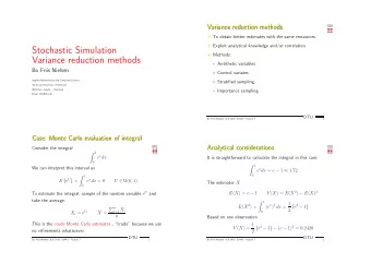
Variance reduction techniques The most efficient way to improve the accuracy and confidence of simulation is to try to reduce the variance of simulation results. We will discuss four different approaches ◮ use of common random variates ◮ use of antithetic random variates ◮ replacing random variables with their expectations ◮ use of control variables
Common random variates Let us study the difference between two system variants ( A and B ). The simulation outputs are X A and X B . We are interested in X A − X B and its expectation α A − α B . The point estimate is ¯ X A − ¯ X B . If the simulations are independent, the variance of the point estimate (difference) is Var ( ¯ X A ) + Var ( ¯ X B ) ≈ ( S 2 A + S 2 B ) / N
Common random variates If simulations are mutually dependent, Var ( ¯ X A − ¯ X B ) = Var ( ¯ X A ) + Var ( ¯ X B ) − 2 Cov ( ¯ X A , ¯ X B ) So, if the simulation experiments are positively correlated, the variance of the result (difference) is smaller than in uncorrelated case. Positive correlation can result from using same random numbers for both variants (arrival times, service times etc generated using same seed values for both variants).
Common random variates ◮ Requires that we can fully control the starting of random streams in every simulation run. ◮ Works best when both variants use the random variates in the same way. ◮ For example, all client related entities are generated at one place independently of clients future path in the system (easy and difficult clients come in same order but are routed differently).
Antithetic variates Consider a single simulation experiment (not a difference of two variants). We use random streams U i , that give N instances of output X i . We then make N additional experiments with random streams U ∗ i with outputs X ∗ i . We choose as point estimate Y = ( ¯ X + ¯ X ∗ ) / 2 for which E ( Y ) = E ( X ) = E ( X ∗ ) and Var ( Y ) = 1 4( Var ( ¯ X ) + Var ( ¯ X ∗ ) + 2 Cov ( ¯ X , ¯ X ∗ )) 2 ( Var ( ¯ X ) + Cov ( ¯ X , ¯ or 1 X ∗ )).
Antithetic variates If Cov ( ¯ X , ¯ X ∗ ) < 0, the variance is reduced more than when doing N independent additional trials. Negative correlation may result from ◮ replacing U by 1 − U in Unif(0,1) generator systematically. ◮ by exchanging the seed values between the arrival time and service time generators etc. This results to making N independent simulations with 2 N simulation runs, so that the extreme phenomena occur in more symmetric way and hence the variance is likely to be smaller.
Replacing with expectations Often the observation of interest is a sum of a random amount of random variates. If the expectation of one of the random variates contributing to the result is known, this can be used in the analysis. Example: Utilixation rate can be defined as N serv � s i / T i =1 where s i is the service time of individual client, N serv the number of clients served. However, we know E ( s i ) (simulation parameter). Let us denote it by t s . Then also N serv t s / T is an estimate for utilization rate.
Replacing with expectations If the system is in equlibrium, then on average clients served = clients arrived - clients lost. Once again we know expectation for clients arrived (simulation parameter t a interarrival time/client) . Thus on average N serv = T / t a − N lost . Hence we get for utilization rate the estimate t s / t a − N lost t s / T This has same expectation but often smaller variance than the original observation.
Replacing with expectations Lost clients can be analyzed further. We lose clients only when they arrive to a full system. Hence E ( N lost ) = E ( T full ) / t a So we can monitor the times when the system is full to get estimate t s / t a (1 − T full / T ) Different estimates do not require new simulation runs (only deeper analysis of the system). It is possible to create several observations and to select the ones that give smallest variances.
Control variables Often the most powerfull way to reduce variance is to use control variables. Control variable is a random variate with known expectation that has strong correlation with the variate of interest. The difference between the control and original variate is to be observed. Let us monitor X i with unknown expectation E ( X i ) = α . In addition we observe Y i with known expectation E ( Y i ) = β . Then the variable V = ¯ X + β − ¯ Y gives an unbiased estimate for α , E ( V ) = α + β − β = α . Var ( V ) = Var ( ¯ X ) + Var ( ¯ Y ) − 2 Cov ( ¯ X , ¯ Y ) If Cov ( ¯ X , ¯ 2 Var ( ¯ Y ) > 1 Y ) then V leads to more accurate estimate to α than X (smaller confidence interval).
Control variables As control variable Y we can use simulation output of a simpler model variant. This requres simulation and theoretical analysis of another model which may be costly and difficult. Another option is to use as Y some model data that is known (expectation) and explains well the quantity of interest). These variables are called concommittant control variables. These do not require additional simulation models or deep analysis. In utilization rate example for example the arrived clients (times average service time) is a control variable for observed total service time.
Recommend
More recommend
Explore More Topics
Stay informed with curated content and fresh updates.


![Variance = E[I 2 ] 2pE[I] + p 2 = E[I] 2p p + p 2 = 2 2 = p-2p+ p pq variance.1](https://c.sambuz.com/1069957/variance-s.webp)
