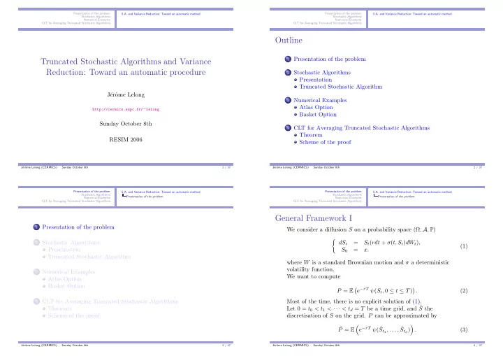
Outline 1 Presentation of the problem Truncated Stochastic - PowerPoint PPT Presentation

Presentation of the problem Presentation of the problem S.A. and Variance Reduction: Toward an automatic method S.A. and Variance Reduction: Toward an automatic method Stochastic Algorithms Stochastic Algorithms Numerical Examples Numerical Examples CLT for Averaging Truncated Stochastic Algorithms CLT for Averaging Truncated Stochastic Algorithms Outline 1 Presentation of the problem Truncated Stochastic Algorithms and Variance Reduction: Toward an automatic procedure 2 Stochastic Algorithms Presentation Truncated Stochastic Algorithm J´ erˆ ome Lelong 3 Numerical Examples Atlas Option http://cermics.enpc.fr/ ∼ lelong Basket Option Sunday October 8th 4 CLT for Averaging Truncated Stochastic Algorithms Theorem RESIM 2006 Scheme of the proof J´ erˆ ome Lelong (CERMICS) Sunday October 8th 1 / 37 J´ erˆ ome Lelong (CERMICS) Sunday October 8th 2 / 37 Presentation of the problem Presentation of the problem S.A. and Variance Reduction: Toward an automatic method S.A. and Variance Reduction: Toward an automatic method Stochastic Algorithms Stochastic Algorithms Presentation of the problem Presentation of the problem Numerical Examples Numerical Examples CLT for Averaging Truncated Stochastic Algorithms CLT for Averaging Truncated Stochastic Algorithms General Framework I 1 Presentation of the problem We consider a diffusion S on a probability space (Ω , A , P ) � dS t 2 Stochastic Algorithms = S t ( rdt + σ ( t, S t ) dW t ) , (1) Presentation S 0 = x. Truncated Stochastic Algorithm where W is a standard Brownian motion and σ a deterministic volatility function. 3 Numerical Examples We want to compute Atlas Option Basket Option � e − rT ψ ( S t , 0 ≤ t ≤ T ) � P = E . (2) 4 CLT for Averaging Truncated Stochastic Algorithms Most of the time, there is no explicit solution of (1). Let 0 = t 0 < t 1 < · · · < t d = T be a time grid, and ˆ Theorem S the Scheme of the proof discretisation of S on the grid. P can be approximated by � � e − rT ψ ( ˆ ˆ S t 1 , . . . , ˆ P = E S t d ) . (3) J´ erˆ ome Lelong (CERMICS) Sunday October 8th 3 / 37 J´ erˆ ome Lelong (CERMICS) Sunday October 8th 4 / 37

Presentation of the problem Presentation of the problem S.A. and Variance Reduction: Toward an automatic method S.A. and Variance Reduction: Toward an automatic method Stochastic Algorithms Stochastic Algorithms Presentation of the problem Presentation of the problem Numerical Examples Numerical Examples CLT for Averaging Truncated Stochastic Algorithms CLT for Averaging Truncated Stochastic Algorithms General Framework II Importance Sampling I An elementary change of variables in the expectation enables to Using standard discretisation schemes, it is quite easy to see that change the mean of G to obtain ψ ( ˆ S t 1 , . . . , ˆ S t d ) can be expressed in terms of the Brownian increments. � � φ ( G + θ ) e − θ · G − � θ � 2 Equation (3) has an equivalent form ˆ P = E (5) 2 ˆ P = E ( φ ( G )) (4) for any θ ∈ R d . where G is a d − dimensional Gaussian vector with identity covariance { X θ = φ ( G + θ ) e − θ · G − � θ � 2 2 ; θ ∈ R d } is of constant expectation. matrix. Find the parameter θ ⋆ that minimises Var( X θ ) Expectation in (4) will be computed using Monte Carlo simulations. The prize is to improve the convergence of the Monte Carlo procedure. rare event simulation : consider φ ( G ) = ( x e σG − K ) + with We focus on Importance Sampling. x ≪ K , P ( { φ ( G ) > 0 } ) may be really small. Centering G + θ around 1 σ ln( K/x ) makes P ( { φ ( G ) > 0 } ) ≈ P ( { φ ( G ) = 0 } ). J´ erˆ ome Lelong (CERMICS) Sunday October 8th 5 / 37 J´ erˆ ome Lelong (CERMICS) Sunday October 8th 6 / 37 Presentation of the problem Presentation of the problem S.A. and Variance Reduction: Toward an automatic method S.A. and Variance Reduction: Toward an automatic method Stochastic Algorithms Stochastic Algorithms Presentation of the problem Stochastic Algorithms Numerical Examples Numerical Examples CLT for Averaging Truncated Stochastic Algorithms CLT for Averaging Truncated Stochastic Algorithms Importance Sampling II 1 Presentation of the problem The variance V is given by 2 Stochastic Algorithms � � � φ ( G + θ ) 2 e − 2 θ · G −� θ � 2 � φ ( G ) 2 e − θ · G + � θ � 2 V ( θ ) = E = E . Presentation 2 Truncated Stochastic Algorithm V is strictly convex and differentiable without any particular 3 Numerical Examples assumptions on ψ , Atlas Option θ ⋆ is also defined as the unique root of ∇ V Basket Option � � ( θ − G ) φ ( G ) 2 e − θ · G + � θ � 2 4 CLT for Averaging Truncated Stochastic Algorithms ∇ V ( θ ) = E = E ( U ( θ, G )) . 2 Theorem Scheme of the proof ⇒ Try to construct a procedure to approximate θ ⋆ . (First = introduced by Arouna [Arouna, 2004]). J´ erˆ ome Lelong (CERMICS) Sunday October 8th 7 / 37 J´ erˆ ome Lelong (CERMICS) Sunday October 8th 8 / 37

Presentation of the problem Presentation of the problem S.A. and Variance Reduction: Toward an automatic method S.A. and Variance Reduction: Toward an automatic method Stochastic Algorithms Stochastic Algorithms Stochastic Algorithms Stochastic Algorithms Numerical Examples Numerical Examples CLT for Averaging Truncated Stochastic Algorithms Presentation CLT for Averaging Truncated Stochastic Algorithms Truncated Stochastic Algorithm Stochastic Algorithms I Truncated Stochastic Algorithm Consider an increasing sequence of compact sets ( K j ) j such that G n i.i.d. ∼ G . � ∞ γ n> 0 , � γ n = ∞ , � γ 2 j =0 K j = R d . n < ∞ . Consider ( G n ) n and ( γ n ) n as defined previously. For θ 0 ∈ R d , Prevent the algorithm from blowing up: θ n +1 = θ n − γ n +1 U ( θ n , G n +1 ) . At each step, θ n should remain in a given compact set. If such is → E ( � U ( θ, G ) � 2 ) increases not the case, reset the algorithm and consider a larger compact This algorithm quickly fails because θ �− much faster than � θ � 2 . set. Need of a more elaborate algorithm. This is due to Chen (see [Chen and Zhu, 1986]). J´ erˆ ome Lelong (CERMICS) Sunday October 8th 9 / 37 J´ erˆ ome Lelong (CERMICS) Sunday October 8th 10 / 37 Presentation of the problem Presentation of the problem S.A. and Variance Reduction: Toward an automatic method S.A. and Variance Reduction: Toward an automatic method Stochastic Algorithms Stochastic Algorithms Stochastic Algorithms Stochastic Algorithms Numerical Examples Numerical Examples CLT for Averaging Truncated Stochastic Algorithms CLT for Averaging Truncated Stochastic Algorithms Truncated Stochastic Algorithm Truncated Stochastic Algorithm For θ 0 ∈ K 0 and σ 0 = 0, we define ( θ n ) n and ( σ n ) n θ ⋆ +  θ n + 1 2 = θ n − γ n +1 U ( θ n , Z n +1 ) ,   2 ∈ K σ n if θ n + 1 θ n +1 = θ n + 1 and σ n +1 = σ n , (6) θ n +1 = θ 0 + + θ n 2   if θ n + 1 2 / ∈ K σ n θ n +1 = θ 0 and σ n +1 = σ n + 1 . θ n +1 = θ n + 1 + σ n counts the number of truncations up to time n . 2 K σ n = K σ n +1 F n = σ ( G k ; k ≤ n ). θ n is F n − measurable and G n +1 is independent of F n . θ n + 1 2 + K σ n +1 = K σ n +1 J´ erˆ ome Lelong (CERMICS) Sunday October 8th 11 / 37 J´ erˆ ome Lelong (CERMICS) Sunday October 8th 12 / 37