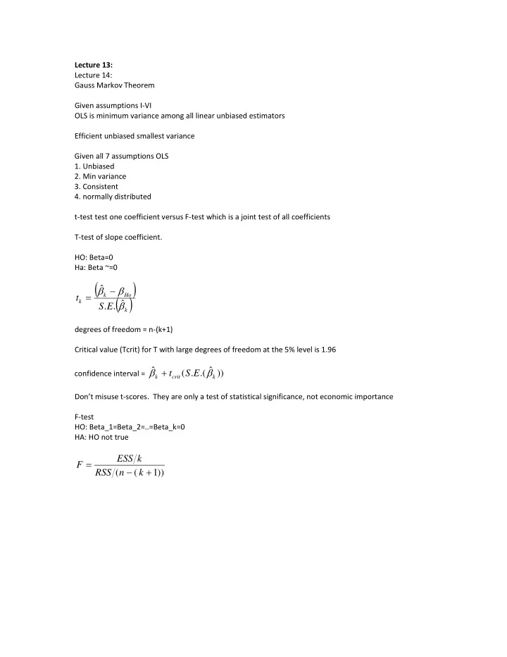
k Ho t k S . E . k degrees of freedom = n - PDF document
Lecture 13: Lecture 14: Gauss Markov Theorem Given assumptions I VI OLS is minimum variance among all linear unbiased estimators Efficient unbiased smallest variance Given all 7 assumptions OLS 1. Unbiased 2. Min variance 3. Consistent 4.
Lecture 13: Lecture 14: Gauss Markov Theorem Given assumptions I ‐ VI OLS is minimum variance among all linear unbiased estimators Efficient unbiased smallest variance Given all 7 assumptions OLS 1. Unbiased 2. Min variance 3. Consistent 4. normally distributed t ‐ test test one coefficient versus F ‐ test which is a joint test of all coefficients T ‐ test of slope coefficient. HO: Beta=0 Ha: Beta ~=0 ˆ k Ho t k ˆ S . E . k degrees of freedom = n ‐ (k+1) Critical value (Tcrit) for T with large degrees of freedom at the 5% level is 1.96 ˆ ˆ t ( S . E .( )) confidence interval = k crit k Don’t misuse t ‐ scores. They are only a test of statistical significance, not economic importance F ‐ test HO: Beta_1=Beta_2=..=Beta_k=0 HA: HO not true ESS k F RSS ( n ( k 1 ))
Examples: From Before: COMMENT lets run our second regression adding yearsdg. REGRESSION /MISSING LISTWISE /STATISTICS COEFF OUTS R /*I've removed the ANOVA from the default */ /CRITERIA=PIN(.05) POUT(.10) /NOORIGIN /DEPENDENT salary /METHOD=ENTER market yearsdg. Model Summary Adjusted R Std. Error of the Model R R Square Square Estimate .824 a 1 .680 .678 7187.88271 a. Predictors: (Constant), yearsdg, market ANOVA b Model Sum of Squares df Mean Square F Sig. .000 a 1 Regression 5.599E10 2 2.799E10 541.813 5.167E7 Residual 2.640E10 511 513 Total 8.239E10 a. Predictors: (Constant), yearsdg, market b. Dependent Variable: salary Coefficients a Standardized Unstandardized Coefficients Coefficients Model B Std. Error Beta t Sig. 2153.797 1 (Constant) -1685.118 -.782 .434 market 39630.458 2131.883 .467 18.589 .000 yearsdg 979.458 34.221 .719 28.622 .000 a. Dependent Variable: salary
A t ‐ test of the slope coefficients for the previous regression would go as follows. For the coefficient on the market variable ˆ k Ho t k ˆ S . E . k T= (39630.458 ‐ 0)/(2131.883) = 18.589 Which is greater than 1.96 so reject HO For the coefficient on the yearsdg variable T= (979.458 ‐ 0)/(34.221) = 28.622 Which is greater than 1.96 so reject HO Remember the F Test ESS k F RSS ( n ( k 1 )) F=( 5.599E10/2)/( 2.640E10/(513-(2+1))) = 541.83 Lecture 15: October 22 EXAM I Chapter 16, 1 ‐ 5
Recommend
More recommend
Explore More Topics
Stay informed with curated content and fresh updates.

