Alex Psomas: Lecture 18. Random Variables: Variance 1. Variance 2. - PowerPoint PPT Presentation
Alex Psomas: Lecture 18. Random Variables: Variance 1. Variance 2. Distributions Variance Flip a coin: If H you make a dollar. If T you lose a dollar. Let X be the RV indicating how much money you make. E ( X ) = 0. Flip a coin: If H you make
Alex Psomas: Lecture 18. Random Variables: Variance 1. Variance 2. Distributions
Variance Flip a coin: If H you make a dollar. If T you lose a dollar. Let X be the RV indicating how much money you make. E ( X ) = 0. Flip a coin: If H you make a million dollars. If T you lose a million dollars. Let Y be the RV indicating how much money you make. E ( Y ) = 0. Any other measures??? What else that’s informative can we say?
Variance The variance measures the deviation from the mean value. Definition: The variance of X is σ 2 ( X ) := var [ X ] = E [( X − E [ X ]) 2 ] . σ ( X ) is called the standard deviation of X .
Variance and Standard Deviation Fact: var [ X ] = E [ X 2 ] − E [ X ] 2 . Indeed: E [( X − E [ X ]) 2 ] var ( X ) = E [ X 2 − 2 XE [ X ]+ E [ X ] 2 ] = E [ X 2 ] − E [ 2 XE [ X ]]+ E [ E [ X ] 2 ] by linearity = E [ X 2 ] − 2 E [ X ] E [ X ]+ E [ X ] 2 , = E [ X 2 ] − E [ X ] 2 . =
Example Consider X with � − 1 , w. p. 0 . 99 X = 99 , w. p. 0 . 01 . Then E [ X ] = − 1 × 0 . 99 + 99 × 0 . 01 = 0 . ( − 1 ) 2 × 0 . 99 +( 99 ) 2 × 0 . 01 ≈ 100 . E [ X 2 ] = Var ( X ) ≈ 100 = ⇒ σ ( X ) ≈ 10 .
A simple example This example illustrates the term ‘standard deviation.’ Consider the random variable X such that � µ − σ , w.p. 1 / 2 X = µ + σ , w.p. 1 / 2 . Then, E [ X ] = µ and E [( X − E [ X ]) 2 ] = σ 2 . Hence, var ( X ) = σ 2 and σ ( X ) = σ .
Properties of variance. 1. Var ( cX ) = c 2 Var ( X ) , where c is a constant. Scales by c 2 . 2. Var ( X + c ) = Var ( X ) , where c is a constant. Shifts center. Proof: E (( cX ) 2 ) − ( E ( cX )) 2 Var ( cX ) = c 2 E ( X 2 ) − c 2 ( E ( X )) 2 = c 2 ( E ( X 2 ) − E ( X ) 2 ) = c 2 Var ( X ) = E (( X + c − E ( X + c )) 2 ) Var ( X + c ) = E (( X + c − E ( X ) − c ) 2 ) = E (( X − E ( X )) 2 ) = Var ( X ) =
Variance of sum of two independent random variables Theorem: If X and Y are independent, then Var ( X + Y ) = Var ( X )+ Var ( Y ) . Proof: Since shifting the random variables does not change their variance, let us subtract their means. That is, we assume that E ( X ) = 0 and E ( Y ) = 0. Then, by independence, E ( XY ) = E ( X ) E ( Y ) = 0 . Var ( X ) = E ( X 2 ) , Var ( Y ) = E ( Y 2 ) . Hence, E (( X + Y ) 2 ) = E ( X 2 + 2 XY + Y 2 ) var ( X + Y ) = E ( X 2 )+ 2 E ( XY )+ E ( Y 2 ) = E ( X 2 )+ E ( Y 2 ) = = var ( X )+ var ( Y ) .
Variance of sum of independent random variables Theorem: If X , Y , Z ,... are pairwise independent, then var ( X + Y + Z + ··· ) = var ( X )+ var ( Y )+ var ( Z )+ ··· . Proof: Since shifting the random variables does not change their variance, let us subtract their means. That is, we assume that E [ X ] = E [ Y ] = ··· = 0. Then, by independence, E [ XY ] = E [ X ] E [ Y ] = 0 . Also, E [ XZ ] = E [ YZ ] = ··· = 0 . Hence, E (( X + Y + Z + ··· ) 2 ) var ( X + Y + Z + ··· ) = E ( X 2 + Y 2 + Z 2 + ··· + 2 XY + 2 XZ + 2 YZ + ··· ) = E ( X 2 )+ E ( Y 2 )+ E ( Z 2 )+ ··· + 0 + ··· + 0 = = var ( X )+ var ( Y )+ var ( Z )+ ··· .
Distributions ◮ Bernoulli ◮ Binomial ◮ Uniform ◮ Geometric
Bernoulli Flip a coin, with heads probability p . Random variable X : 1 is heads, 0 if not heads. X has the Bernoulli distribution. Distribution: � 1 w.p. p X = w.p. 1 − p 0 E [ X ] = p E [ X 2 ] = 1 2 × p + 0 2 × ( 1 − p ) = p Var [ X ] = E [ X 2 ] − ( E [ X ]) 2 = p − p 2 = p ( 1 − p ) Notice that: p = 0 = ⇒ Var ( X ) = 0 p = 1 = ⇒ Var ( X ) = 0
Jacob Bernoulli
Binomial Flip n coins with heads probability p . Random variable: number of heads. Binomial Distribution: Pr [ X = i ] , for each i . How many sample points in event “ X = i ”? � n � i heads out of n coin flips = ⇒ i Sample space: Ω = { HHH ... HH , HHH ... HT ,... } What is the probability of ω if ω has i heads? Probability of heads in any position is p . Probability of tails in any position is ( 1 − p ) . So, we get Pr [ ω ] = p i ( 1 − p ) n − i . Probability of “ X = i ” is sum of Pr [ ω ] , ω ∈ “ X = i ”. � n � p i ( 1 − p ) n − i , i = 0 , 1 ,..., n : B ( n , p ) distribution Pr [ X = i ] = i
Expectation of Binomial Distribution Indicator for the i -th coin: � 1 if i th flip is heads X i = 0 otherwise E [ X i ] = 1 × Pr [“ heads ′′ ]+ 0 × Pr [“ tails ′′ ] = p . Moreover X = X 1 + ··· X n and E [ X ] = E [ X 1 ]+ E [ X 2 ]+ ··· E [ X n ] = n × E [ X i ]= np .
Variance of Binomial Distribution. � 1 if i th flip is heads X i = 0 otherwise i ) = 1 2 × p + 0 2 × ( 1 − p ) = p . E ( X 2 Var ( X i ) = p − ( E ( X i )) 2 = p − p 2 = p ( 1 − p ) . X = X 1 + X 2 + ... X n . X i and X j are independent: Pr [ X i = 1 | X j = 1 ] = Pr [ X i = 1 ] . Var ( X ) = Var ( X 1 + ··· X n ) = np ( 1 − p ) .
Uniform Distribution Roll a six-sided balanced die. Let X be the number of pips (dots). Then X is equally likely to take any of the values { 1 , 2 ,..., 6 } . We say that X is uniformly distributed in { 1 , 2 ,..., 6 } . More generally, we say that X is uniformly distributed in { 1 , 2 ,..., n } if Pr [ X = m ] = 1 / n for m = 1 , 2 ,..., n . In that case, n n m × 1 n = 1 n ( n + 1 ) = n + 1 ∑ ∑ E [ X ] = mPr [ X = m ] = . n 2 2 m = 1 m = 1
Variance of Uniform E [ X ] = n + 1 . 2 Also, n n i 2 Pr [ X = i ] = 1 E [ X 2 ] i 2 ∑ ∑ = n i = 1 i = 1 1 + 3 n + 2 n 2 = , as you can verify. 6 This gives = n 2 − 1 var ( X ) = 1 + 3 n + 2 n 2 − ( n + 1 ) 2 . 6 4 12
Geometric Distribution Let’s flip a coin with Pr [ H ] = p until we get H . For instance: ω 1 = H , or ω 2 = T H , or ω 3 = T T H , or ω n = T T T T ··· T H . Note that Ω = { ω n , n = 1 , 2 ,... } . Let X be the number of flips until the first H . Then, X ( ω n ) = n . Also, Pr [ X = n ] = ( 1 − p ) n − 1 p , n ≥ 1 .
Geometric Distribution Pr [ X = n ] = ( 1 − p ) n − 1 p , n ≥ 1 .
Geometric Distribution Pr [ X = n ] = ( 1 − p ) n − 1 p , n ≥ 1 . Note that ∞ ∞ ∞ ∞ ( 1 − p ) n − 1 = p ( 1 − p ) n − 1 p = p ( 1 − p ) n . ∑ ∑ ∑ ∑ Pr [ X = n ] = n = 1 n = 1 n = 1 n = 0 n = 0 a n for | a | < 1. S = We want to analyze S := ∑ ∞ 1 1 − a . Indeed, 1 + a + a 2 + a 3 + ··· S = a + a 2 + a 3 + a 4 + ··· aS = 1 + a − a + a 2 − a 2 + ··· = 1 . ( 1 − a ) S = Hence, ∞ 1 ∑ Pr [ X = n ] = p 1 − ( 1 − p ) = 1 . n = 1
Geometric Distribution: Expectation X ∼ Geom ( p ) , i.e., Pr [ X = n ] = ( 1 − p ) n − 1 p , n ≥ 1 . One has ∞ ∞ n ( 1 − p ) n − 1 p . ∑ ∑ E [ X ] = nPr [ X = n ] = n = 1 n = 1 Thus, p + 2 ( 1 − p ) p + 3 ( 1 − p ) 2 p + 4 ( 1 − p ) 3 p + ··· E [ X ] = ( 1 − p ) p + 2 ( 1 − p ) 2 p + 3 ( 1 − p ) 3 p + ··· ( 1 − p ) E [ X ] = p + ( 1 − p ) p + ( 1 − p ) 2 p + ( 1 − p ) 3 p + ··· pE [ X ] = by subtracting the previous two identities ∞ ∞ ( 1 − p ) n − 1 p = ∑ ∑ = Pr [ X = n ] = 1 . n = 1 n = 1 Hence, E [ X ] = 1 p .
Coupon Collectors Problem. Experiment: Get coupons at random from n until collect all n coupons. Outcomes: { 123145 ..., 56765 ... } Random Variable: X - length of outcome. Before: Pr [ X ≥ n ln2 n ] ≤ 1 2 . Today: E [ X ] ?
Time to collect coupons X -time to get n coupons. X 1 - time to get first coupon. Note: X 1 = 1. E ( X 1 ) = 1 . X 2 - time to get second (distinct) coupon after getting first. Pr [ “get second distinct coupon” | “got first coupon ′′ ] = n − 1 n ⇒ E [ X 2 ] = 1 1 n E [ X 2 ]? Geometric ! ! ! = p = = n − 1 . n − 1 n Pr [ “getting i th distinct coupon | “got i − 1 distinct coupons” ] = n − ( i − 1 ) = n − i + 1 n n E [ X i ] = 1 n p = n − i + 1 , i = 1 , 2 ,..., n . E [ X 1 ]+ ··· + E [ X n ] = n n n − 2 + ··· + n n E [ X ] = n + n − 1 + 1 n ( 1 + 1 2 + ··· + 1 = n ) =: nH ( n ) ≈ n ( ln n + γ )
Review: Harmonic sum � n H ( n ) = 1 + 1 2 + ··· + 1 1 n ≈ x dx = ln ( n ) . 1 . A good approximation is H ( n ) ≈ ln ( n )+ γ where γ ≈ 0 . 58 (Euler-Mascheroni constant).
Harmonic sum: Paradox Consider this stack of cards (no glue!): If each card has length 2, the stack can extend H ( n ) to the right of the table. As n increases, you can go as far as you want!
Stacking The cards have width 2. Induction shows that the center of gravity after n cards is H ( n ) away from the right-most edge.
Geometric Distribution: Memoryless Let X be Geom ( p ) . Then, for n ≥ 0, Pr [ X > n ] = Pr [ first n flips are T ] = ( 1 − p ) n . Theorem Pr [ X > n + m | X > n ] = Pr [ X > m ] , m , n ≥ 0 . Proof: Pr [ X > n + m and X > n ] Pr [ X > n + m | X > n ] = Pr [ X > n ] Pr [ X > n + m ] = Pr [ X > n ] ( 1 − p ) n + m = ( 1 − p ) m = ( 1 − p ) n = Pr [ X > m ] .
Geometric Distribution: Memoryless - Interpretation Pr [ X > n + m | X > n ] = Pr [ X > m ] , m , n ≥ 0 . The coin is memoryless, therefore, so is X .
Geometric Distribution: Yet another look Theorem: For a r.v. X that takes the values { 0 , 1 , 2 ,... } , one has ∞ ∑ E [ X ] = Pr [ X ≥ i ] . i = 1 [See later for a proof.] If X = Geom ( p ) , then Pr [ X ≥ i ] = Pr [ X > i − 1 ] = ( 1 − p ) i − 1 . Hence, ∞ ∞ 1 − ( 1 − p ) = 1 1 ( 1 − p ) i − 1 = ( 1 − p ) i = ∑ ∑ E [ X ] = p . i = 1 i = 0
Recommend
More recommend
Explore More Topics
Stay informed with curated content and fresh updates.

![Alex Psomas: Lecture 15. Conditional Probability: Review Monty Hall Recall: Pr [ A | B ] =](https://c.sambuz.com/996856/alex-psomas-lecture-15-conditional-probability-review-s.webp)




![variance Var[ X ] = E[( X - ) 2 ], often denoted 2 . The standard deviation of X is =](https://c.sambuz.com/996498/variance-s.webp)
