Statistics I Chapter 5 Discrete Probability Distributions - PowerPoint PPT Presentation

Statistics I – Chapter 5, Fall 2012 1 / 70 Statistics I – Chapter 5 Discrete Probability Distributions Ling-Chieh Kung Department of Information Management National Taiwan University October 3, 2012

Statistics I – Chapter 5, Fall 2012 2 / 70 Introduction ◮ We have studied frequency distributions . ◮ For each value or interval, what is the frequency? ◮ In the next three chapters, we will study probability distributions . ◮ For each value or interval, what is the probability? ◮ There are two types of probability distribution: ◮ Population distributions: Chapters 5 and 6. ◮ Sampling distributions: Chapter 7.

Statistics I – Chapter 5, Fall 2012 3 / 70 Random variables Basic concepts Road map ◮ Random variables . ◮ Basic concepts. ◮ Expectations and variances. ◮ Binomial distributions. ◮ Hypergeometric distributions. ◮ Poisson distributions.

Statistics I – Chapter 5, Fall 2012 4 / 70 Random variables Basic concepts Random variables ◮ A random variable (RV) is a variable whose outcomes are random. ◮ Examples: ◮ The outcome of tossing a coin. ◮ The outcome of rolling a dice. ◮ The number of people preferring Pepsi to Coke in a group of 25 people. ◮ The number of consumers entering a bookstore at 7-8pm. ◮ The temperature of this classroom at tomorrow noon. ◮ The average studying hours of a group of 10 students.

Statistics I – Chapter 5, Fall 2012 5 / 70 Random variables Basic concepts Discrete random variables ◮ A random variable can be discrete, continuous, or mixed. ◮ A random variable is discrete if the set of all possible values is finite or countably infinite . ◮ The outcome of tossing a coin: Finite. ◮ The outcome of rolling a dice: Finite. ◮ The number of people preferring Pepsi to Coke in a group of 25 people: Finite. ◮ The number of consumers entering a bookstore at 7-8pm: Countably infinite.

Statistics I – Chapter 5, Fall 2012 6 / 70 Random variables Basic concepts Continuous random variables ◮ A random variable is continuous if the set of all possible values is uncountable. ◮ The temperature of this classroom at tomorrow noon. ◮ The average studying hours of a group of 10 students. ◮ The interarrival time between two consumers. ◮ The GDP per capita of Taiwan in 2013.

Statistics I – Chapter 5, Fall 2012 7 / 70 Random variables Basic concepts Discrete v.s. continuous RVs ◮ For a discrete RV, typically things are counted . ◮ Typically there are gaps among possible values. ◮ For a continuous RV, typically things are measured . ◮ Typically possible values form an interval . ◮ Such an interval may have a infinite length. ◮ Sometimes a random variable is called mixed . ◮ On Saturday I may or may not go to school. If I go, I need at least one hour for communication. Let X be the number of hours I spend in working including communication on Saturday. Then X ∈ { 0 } ∪ [1 , 24]. ◮ By definition, is a mixed RV discrete or continuous?

Statistics I – Chapter 5, Fall 2012 8 / 70 Random variables Basic concepts Discrete and continuous distributions ◮ The possibilities of outcomes of a random variable are summarized by probability distributions , or simply distributions. ◮ As variables can be either discrete or continuous, distributions may also be either discrete or continuous. ◮ In this chapter we study discrete distributions. ◮ In Chapter 6 we study continuous distributions.

Statistics I – Chapter 5, Fall 2012 9 / 70 Random variables Basic concepts Describing a discrete distribution ◮ On way to fully describe a discrete distribution is to list all possible outcomes and their probabilities. ◮ Let X be the result of tossing a fair coin: x H T 1 1 Pr( X = x ) 2 2 ◮ Let X be the result of rolling a fair dice: x 1 2 3 4 5 6 1 1 1 1 1 1 Pr( X = x ) 6 6 6 6 6 6

Statistics I – Chapter 5, Fall 2012 10 / 70 Random variables Basic concepts Describing a discrete distribution ◮ But complete enumeration is unsatisfactory if there are too many (or even infinite) possible values. ◮ Also, sometimes there is a formula for the probabilities. ◮ Suppose we toss a fair coin and will stop with a tail. ◮ Let X be the number of tosses we make. ◮ Pr( X = 1) = 1 2 (getting a tail at the first time). ◮ Pr( X = 2) = ( 1 2 )( 1 2 ) = 1 4 (head and then a tail). ◮ Pr( X = 3) = ( 1 2 )( 1 2 )( 1 2 ) = 1 8 (head, head, and then a tail). 2 ) x for all x = 1 , 2 , ... . ◮ In general, Pr( X = x ) = ( 1 ◮ No need to create a table!

Statistics I – Chapter 5, Fall 2012 11 / 70 Random variables Basic concepts Probability mass functions ◮ The formula of calculating the probability of each possible value of a discrete random variable is call a probability mass function (pmf). ◮ This is sometimes abbreviated as a probability function (pf). ◮ Pr( X = x ) = ( 1 2 ) x , x = 1 , 2 , ... , is the pmf of X . ◮ If the meaning is clear, Pr( X = x ) is abbreviated as Pr( x ). ◮ Any finite list of probabilities can be described by a pmf. ◮ In practice, many random variables cannot be exactly described by a pmf (or the pmf is too hard to be found). ◮ In this case, people may approximate the distribution of the random variable by a distribution with a known pmf. ◮ So the first step is to study some well-known distributions.

Statistics I – Chapter 5, Fall 2012 12 / 70 Random variables Basic concepts Parameters of a distribution ◮ A distribution depends on a formula. ◮ A formula depends on some parameters . ◮ Suppose the coin now generates a head with probability p . ◮ How to modify the original pmf Pr( X = x ) = ( 1 2 ) x ? ◮ The pmf becomes Pr( X = x | p ) = p x − 1 (1 − p ), x = 1 , 2 , ... . ◮ The probability p is called the parameter of this distribution. ◮ Be aware of the difference between: ◮ The parameter of a population and ◮ The parameter of a distribution.

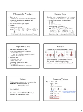
Statistics I – Chapter 5, Fall 2012 13 / 70 Random variables Expectations and variances Descriptive measures ◮ Consider a discrete random variable X with a sample space S , realizations { x i } i ∈ S , and a pmf Pr( · ). ◮ The expected value (or mean) of X is � µ ≡ E [ X ] = x i Pr( x i ) . i ∈ S ◮ The variance of X is � σ 2 ≡ Var( X ) ≡ E ( x i − µ ) 2 Pr( x i ) . � ( X − µ ) 2 � = i ∈ S √ ◮ The standard deviation of X is σ ≡ σ 2 .

Statistics I – Chapter 5, Fall 2012 14 / 70 Random variables Expectations and variances Descriptive measures: an example ◮ Let X be the outcome of rolling a dice, then the pmf is Pr( x ) = 1 6 for all x = 1 , 2 , ..., 6. ◮ The expected value of X is 6 x i Pr( x i ) = 1 � E [ X ] ≡ 6(1 + 2 + · · · + 6) = 3 . 5 . i =1 ◮ The variance of X is � ( x i − µ ) 2 Pr( x i ) Var( X ) ≡ i ∈ S = 1 � ( − 2 . 5) 2 + ( − 1 . 5) 2 + · · · + 2 . 5 2 � ≈ 2 . 92 . 6 √ ◮ The standard deviation of X is 2 . 92 ≈ 1 . 71.

Statistics I – Chapter 5, Fall 2012 15 / 70 Random variables Expectations and variances Linear functions of a random variable ◮ Consider the linear function a + bX of a RV X . Proposition 1 Let X be a random variable and a and b be two known constants, then Var( a + bX ) = b 2 Var( X ) . E [ a + bX ] = a + b E [ X ] and Proof. Similar to Problems 5a and 5b in Homework 3. ◮ If one earns 5 x by rolling x , the expected value of variance of the earning of rolling a dice are 17 . 5 and 72 . 92.

Statistics I – Chapter 5, Fall 2012 16 / 70 Random variables Expectations and variances Expectation of a sum of RVs ◮ Consider the sum of a set of n random variables: n � X i = X 1 + X 2 + · · · + X n . i =1 What is the expectation? ◮ “Expectation of a sum is the sum of expectations:” Proposition 2 Let { X i } i =1 ,...,n be a set of random variables, then � � n n � � E X i = E [ X i ] . i =1 i =1

Statistics I – Chapter 5, Fall 2012 17 / 70 Random variables Expectations and variances Expectation of a sum of RVs ◮ Proof of Proposition 2. Suppose n = 2 and S i is the sample space of X i , then � � E [ X 1 + X 2 ] = ( x 1 + x 2 ) Pr( x 1 , x 2 ) x 1 ∈ S 1 x 2 ∈ S 2 � � � � = x 1 Pr( x 1 , x 2 ) + x 2 Pr( x 1 , x 2 ) x 1 ∈ S 1 x 2 ∈ S 2 x 2 ∈ S 1 x 1 ∈ S 2 � � � � = x 1 Pr( x 1 , x 2 ) + x 2 Pr( x 1 , x 2 ) x 1 ∈ S 1 x 2 ∈ S 2 x 2 ∈ S 2 x 1 ∈ S 1 � � = x 1 Pr( x 1 ) + x 2 Pr( x 2 ) = E [ X 1 ] + E [ X 2 ] , x 1 ∈ S 1 x 2 ∈ S 2 where Pr( x 1 , x 2 ) is the abbreviation of Pr( X 1 = x 1 , X 2 = x 2 ).

Statistics I – Chapter 5, Fall 2012 18 / 70 Random variables Expectations and variances Expectation of a product of RVs ◮ Consider the product of n independent random variables: n � X i = X 1 × X 2 × · · · × X n . i =1 Proposition 3 Let { X i } i =1 ,...,n be a set of independent RVs, then � � n n � � X i = E [ X i ] . E i =1 i =1 Proof. Homework!

Statistics I – Chapter 5, Fall 2012 19 / 70 Random variables Expectations and variances Variance of sum of RVs ◮ “Variance of an independent sum is the sum of variances:” Proposition 4 Let { X i } i =1 ,...,n be a set of independent random variables, then � � n n � � Var = Var( X i ) . X i i =1 i =1 ◮ Is Var(2 X ) = 2Var( X )? Why? ◮ Is E (2 X ) = 2 E ( X )? Why?